Preference Models With Latent Variables Research Paper

The prevalence of behavioral models with their objective of choice prediction originated with the work of Thurstone (1927). By invoking the psychophysical concept of a sensory continuum, Thurstone explained the observation that choices by the same person may not be deterministic under seemingly identical conditions. He argued that options should be represented along this sensory continuum by random variables that describe the options’ effects on a person’s sensory apparatus. The choice process is then reduced to selecting the option with the greatest realization. One may question the use of randomness as a device to represent factors that determine the formation of preferences but are unknown to the observer. However, because, in general, it is not feasible to identify or measure all relevant choice determinants (such as all attributes of the choice options of the person choosing, or of environmental factors) the question of whether the choice process is inherently random or is determined by a multitude of different factors may be of little relevance in at least one aspect: either position arrives at the same conclusion that choices are best described in terms of their probabilities of occurrence.

Thurstone’s early conceptualizations gave rise to an extensive body of methodological and empirical research, mainly in economics and psychology. Surveys about developments in choice theories (e.g. see Decision and Choice: Random Utility Models of Choice and Response Time; Luce’s Choice Axiom; Ranking Models, Mathematics of, Marley 1992, Suppes et al. 1992) and choice modeling (Amemiya 1985, Fligner and Verducci 1993, Manski and McFadden 1981, McFadden 1984) indicate that the merging of the literatures in these two disciplines produced a flexible and powerful framework for the structural investigation of choice data. In particular, this framework has proved to be useful for analyses of individual preference differences at a particular point in time and over time, multidimensional representations of choice alternatives, and the incorporation of variables that describe choice options and decision makers. Each of these areas of research is outlined in the following sections. Because emphasis is on conceptual issues, more technical topics such as sampling, estimation and inference will not be discussed (Albert and Chib 1993).

2. Theoretical Framework

We define a population P of decision makers (n ϵ P) and a finite set l of choice alternatives ( j ϵ l). For each decision maker n and choice alternative j, a vector x_nj of observed variables is available that partially describe the pair (n, j ). The underlying momentary utility of option j to person n is denoted by u_nj and a function of the observed and unobserved attribute values. Distributional assumptions are made to capture the variation of the unobserved attribute values and taste differences among the decision makers. In combination with a decision rule for selecting an option, the utilities determine the options’ choice probabilities. As a result, the choice probabilities can be represented by an a priori specified member of a family of functions which is partially determined by the distributional assumptions about the unobserved attribute values and utility variations and indexed by a parameter vector θ.

Choice data may be collected in a variety of formats. For example, the paired comparison technique is the method of choice in laboratory settings. In large scale surveys or panel interviewer studies, incomplete and/or partial rankings or preference ratings are frequently collected because of their time-efficiency. In conjoint measurement studies (e.g., see Measurement Theory: Conjoint), the constant-sum technique is often used. In recurrent choice studies, we observe how often each choice option is selected within a certain time period. Each data type requires a different treatment to both investigate how decision makers differ in their preferences for choice options and to accommodate the distinct psychological processes that are specific to each choice task.

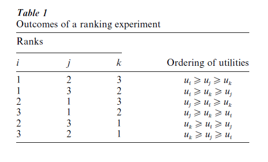
Consider, for example, a ranking experiment with the choice set l = {i, j, k} but without any attribute information. The first three columns of Table 1 represent the six possible ranking outcomes. Each number corresponds to one of the ranking positions of an option. For instance, the ranking outcome {2, 1, 3} indicates that options i, j and k are ranked second, first and third, respectively. Here the rankings are obtained based on the ordering (from largest to smallest) of the underlying options’ utilities. The remaining columns of Table 1 depict these orderings of the utility values (without the subscript n) for each of the six ranking outcomes. For instance, u_j ≥ u_i ≥ u_k indicates that the utility of j is larger than the utility of i which, in turn, is larger than the utility of k. The probability of observing this ranking outcome can be written as Pr( j ≥ i ≥ k|θ) = Pr[(u_j – u_i) ≥ 0 (u_i – u_k) ≥ 0]. If the individual utilities follow a multivariate normal distribution with mean vector µ = ( µ_i, µ_j, µ_k) and covariance matrix

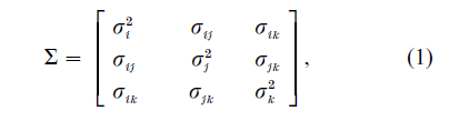
then probability of observing this ranking can be computed by evaluating the cumulative distribution function of the bivariate normal density with upper integration limits ( µ_j – µ_i) (σ_j² – 2σ_ij + σ_i²) and ( µ_i – µ_k) / (σ_i² -2σ_ik +σ²_k) and correlation coefficient (σ_ij – σ_jk -σ_i² + σ_ik)[(σ_j² – 2σ_ij + σ_i²)^1/2(σ_i² – 2σ_ik + σ_k²)^1/2]^-1. It is important to note that because the ranking probabilities are based on the differences between the options’ utilities, it is not possible to uniquely identify the underlying mean and covariance structure.

When relating attribute information to individual utilities, it is useful to distinguish between systematic and random sources of influence. Random sources of influence include (a) attributes of the choice options that are unobserved but influence preferences, (b) measurement errors, and (c) unobserved variables that account for taste variations among the decision makers (Manski & McFadden 1981). Systematic components of influence include the effects of the measured person and option characteristics x_nj. The implication of this view is that u_nj can be written as u_nj = µ_nj + ε_nj, where µ_nj and ε_nj represent the effects of observed and unobserved determinants, respectively, of an option’s utility. Without prior information, we can only determine the distribution of the unobserved values across the population of decision makers.

2.1 Modeling µ

The specific functional relationship between µ_nj and known option and person characteristics may depend on the particular application. For example, in situations where the measured attributes of the choice options are of a ‘more-is-better’ type, a linear function may prove sufficient to describe the attributes’ effects. This is the case for the vector model (Carroll and DeSoete 1991) which assumes that a decision maker combines the attribute values in a linear fashion. In contrast, when the systematic utility component is a single-peaked function of the measured variables, an ideal-point representation is more appropriate (Coombs 1964).

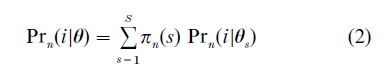
The attribute effects may vary from person to person in a systematic fashion, for example, by being related to such person-specific variables as age, gender, and educational achievement. However, in many cases reference to demographic variables is not sufficient to explain heterogeneity in preferences among individuals. Because psychological or economic theories provide little guidance about the role person-specific variables play in the formation of preferences, a random regression approach is required. Thus, it may be postulated that the attribute effects follow some a priori specified distribution. In particular, latent structure models are useful in capturing individual differences in the attribute effects by introducing the fairly unrestrictive assumption that individual variations can be described by a small number of ‘prototypical’ effect vectors (Bockenholt and Bockenholt 1991). Individual differences are accounted for by assigning each person to a preference class such that members of a preference class exhibit the same or similar attribute effects. For example, when preference data are collected by the method of first choices, a latent-class choice model is given by the following equation

where

• Pr_n(i|θ) = probability of person n choosing alternative i, and θ is a parameter vector;
• π_n(s) = probability of person n belonging to class s;
• Pr_n(i|θ_s) = probability of person n choosing alternative i given n belonging to class s.

The latent classes may represent (a) different decision rules adopted by the individuals; (b) variable choice sets considered by the individuals; or (c) subgroups of the population with varying tastes or, sensitivity to the options and their attributes.

2.2 Modeling ε

Attributes that influence the utility of an alternative but are not measured are represented by ε_j. The distribution of ε_j is frequently specified to be multivariate normal with arbitrary covariance matrix. This specification is useful in analyzing similarity relationships between choice options that are introduced by the unmeasured attributes. Because the estimation of the elements of the covariance matrix is computationally complex, more restrictive representations are also of interest. For example, Stern (1990) proposed a family of choice models based on independent gamma random variables which includes Luce’s (1959) choice model as a special case.

Careful checks are necessary to determine whether the independence assumption is valid or whether unobserved attributes may contain information useful in identifying systematic sources of individual differences and option characteristics. If respondents perceive a common set of latent attributes but differ in the weights they assign to the attribute values, the covariances of ε_j can be decomposed according to a linear factor-analytic model (Takane 1987). Other possibilities include the application of ideal-point models which are based on the assumption that individuals choose the option that is closest to their ‘ideal option’ where closeness is a function of the distance between the choice option and the person-specific ideal option (Coombs 1964). Distance may be defined in various ways, for example, by an Euclidean distance in a continuous latent attribute space or by a latent tree structure in which both choice and ‘ideal’ options are represented by nodes. However, in all of these cases, the interpretation of taste differences is much simplified provided the assumption is correct that decision makers use the same set of attributes in assessing the choice options.

2.3 Modeling Preferences Over Time

When collecting time-dependent choice data, it is important to take into account that individuals not only differ in their preferences at a particular point in time but also in the way they change their preferences over time. For instance, current preferences may depend on such diverse factors as previous choices, interchoice times, or the length of time a particular preference state has been occupied. Decision makers may also differ in their familiarity with features of the choice options with the result that some decision makers are stable in their preferences over time while others may change their preferences according to some learning process. A complicating factor in this context is that choice environments outside a laboratory setting are rarely stable. Typically, attributes of choice options (e.g., price) and decision environments (e.g., changing tax code) vary over time and influence choice behavior.

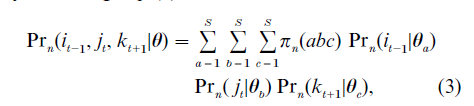
The development of time-dependent choice models requires significant modifications of the statistical framework for cross-sectional choice data. However, because choice processes are inherently dynamic and are studied best by taking their temporal nature into account, approaches that focus on these aspects are more likely to lead to important insights about decision making. Conceptually, it is useful to distinguish between heterogeneity and state dependence in the analysis of recurrent choice data. According to the ‘heterogeneity approach,’ individual choices are assumed to be conditionally independent given the person-specific parameters. For example, latent structure choice models represent time-dependent individual differences by switches among latent preference states. If preferences are stable, membership in a latent preference state is time-homogeneous. In contrast, systematic choice variability over time may indicate changes in the perception of (some of ) the choice options. Stability and shifts in preference states (for, say, three equidistant time points) can be investigated by extending Eq. (2) to

where

• Pr_n(i_t−1, j_t, k_t+1|θ) = probability of person n choosing alternative i at time point (t-1), j at time point t, and k at time point (t+1); and
• π_n(abc) = probability of person n belonging to classes a, b, and c at time points (t-1), t, and t+1, respectively.

Special cases of (3) are obtained by imposing constraints on πn(abc) to describe the switching process among the latent preference states (Bockenholt and Langeheine 1996).

Although time-varying taste heterogeneity is perhaps the single most important source of dependency in recurrent choice data, the assumption of conditionally independent decisions may require the estimation of a large number of preference states in order to be satisfied. A more parsimonious approach for modeling state dependency is obtained by considering the outcomes of previous choices as possible explanatory variables for current choices. For example, if only the choice outcome at (t-1) influences the current choice, the state-specific choice probabilities are specified as Pr_n( j_t|i_t−1, θ_s). This approach has been shown to be fruitful in capturing such psycho-logical phenomena as habit persistence, learning, or variety seeking (Manski and McFadden 1981). Further generalizations are also possible by allowing for several sets of preference states, where each set follows a different switching process over time.

3. Conclusion

The formulation of choice models in terms of latent utilities has a long tradition in biometric, econometric, psychometric and sociometric disciplines. The numerous applications and further developments in each of these areas have led to many improvements in the statistical apparatus necessary for estimating and validating choice models. However, the unifying principle remains valid that observed individual choice behavior is an imperfect reflection of the underlying preferences of a person. This viewpoint leads to a probabilistic representation of the relation between the manifest and latent levels of choice analysis taking into account both the process by which an individual arrives at a choice and the factors that influence this process. Some of these factors are unobservable (such as the processed information about the choice alternatives), while other factors are known and measurable. By separating these two sources of influence due to measured and unobserved attributes at the individual level, a powerful modeling approach is obtained that facilitates the identification and isolation of the net effects of choice option characteristics, individual characteristics, and interactions of option and individual characteristics as separate choice determinants.

Modifications of this choice modeling approach are necessary when the choice set is large or when a simultaneous presentation of the choice options is not feasible. In these cases, one may argue that decision makers tend to rely on satisfying rules and the idea of an aspiration le el may be more appropriate than the principle of utility maximization (Simon 1957). In contrast to the large number of possible satisfying rules, however, only a few mathematical representations have been proposed. Perhaps the most popular model is due to Coombs’ (1964) analysis of the ‘pick any m’ task and Thurstone’s (1959) work on the method of successive categories. In the ‘pick any m’ task it is assumed that choice options are selected when their utilities exceed some specified minimum value. Thus, the underlying choice process is scalar valued and based on a binary comparison between the option’s utility and a threshold value. More specifically, according to Coombs’ (1964) unidimensional unfolding approach, the utility of item j for person n is given by the distance between two parameters representing j and n on a unidimensional continuum. This idea has been incorporated in several psychometric models by making the simplifying assumption that the perception of the item-specific parameters does not vary from person to person (Andrich 1997). In general, results of the maximization and ‘aspiration level’ hypotheses are not directly comparable because in the latter case we model the probability of belonging to some category (i.e., ‘above the threshold’) and in the former case we model order relations among the choice options.

In recent years, stochastic choice models have come under criticism because, frequently, they cannot capture context-sensitive behavior (Tversky and Kahneman 1991). For example, the models’ under- lying assumption that the assessment of an option’s utility does not depend on comparisons drawn be-tween it and other available alternatives has received little support in laboratory studies. Moreover, the deliberation process from the onset of the choice task to the final selection has been shown to play an important role that should be taken into account by the next generation of choice models (Busemeyer and Townsend 1993). Clearly, the latent utility approach has proved to be most useful in providing parsimonious descriptions of how judges differ in their preferences at a particular point in time or over time. However, by emphasizing interindividual differences, this approach can render only limited insights about cognitive processes influencing a choice.

Bibliography:

1. Albert J, Chib S 1993 Bayesian analysis of binary and polychotomous data. Journal of the American Statistical Association 88: 669–79
2. Amemiya T 1985 Advanced Econometrics. Harvard University Press, Cambridge, MA
3. Andrich D 1997 A hyperbolic cosine IRT model for unfolding direct responses of persons to items. In: van der Linden W J, Hambleton R K (eds.) Handbook of Modern Item Response Theory. Springer, New York, pp. 319–414
4. Bockenholt U, Bockenholt I 1991 Constrained latent class analysis: Simultaneous classification and scaling of discrete choice data. Psychometrika 56: 699–716
5. Bockenholt U, Langeheine R 1996 Latent change in recurrent choice data. Psychometrika 61: 285–302
6. Busemeyer J R, Townsend J T 1992 Decision field theory: A dynamic cognition approach to decision making. Psychological Review 100: 432–59
7. Carroll J D, DeSoete G 1991 Toward a new paradigm for the study of multiattribute choice behavior. American Psychologist 46: 342–52
8. Coombs C 1964 A Theory of Data. Wiley, New York
9. Fligner M A, Verducci J S (eds.) 1993 Probability Models and Statistical Analyses for Ranking Data. Springer, New York
10. Luce R D 1959 Individual Choice Behavior. Wiley, New York
11. Manski C F, McFadden D (eds.) 1981 Structural Analysis of Discrete Data with Econometric Applications. MIT Press, Cambridge, MA
12. Marley A A J 1992 A selective review of recent characterizations of stochastic choice models using distribution and functional equation techniques. Mathematical Social Sciences 23: 5–30
13. McFadden D 1984 Qualitative choice models. In: Griliches Z, Intriligator M D (eds.) Handbook of Econometrics. MIT Press: Cambridge, Vol. II, pp. 1395–457
14. Simon H A 1957 Models of Man: Social and Rational, Mathematical essays on rational human behavior in a social setting. Wiley, New York
15. Stern H 1990 A continuum of paired comparison models. Biometrika 77: 265–73
16. Suppes P, Krantz D, Luce D, Tversky A 1992 Foundation of Measurement. Geometric, Threshold, and Probabilistic Representations. Academic Press, San Diego, Vol. II
17. Takane Y 1987 Analysis of covariance structures and probabilistic binary choice data. Communication and Cognition 20: 45–62
18. Thurstone L L 1927 A law of comparative judgment. Psycho- logical Review 34: 273–86
19. Thurstone L L 1959 The Measurement of Values. University of Chicago Press, Chicago
20. Tversky A, Kahneman D 1991 Loss aversion in riskless choice: A reference-dependent model. Quarterly Journal of Economics 107: 1039–61