Multidimensional Scaling In Psychology Research Paper

In nonmetric MDS only the rank orders of proximities are used. In one widely cited example, the map of 10 US cities was reconstructed so well, using the rank orders of pairwise distances from a table of airline distances, that the map could be almost perfectly superimposed on a standard map of the United States, once the scale factor was adjusted appropriately, and a rigid rotation was applied to the MDS map to align its coordinates with the north–south and east–west coordinates of the standard map.

Rotation of coordinates is not a trivial issue (at least when Euclidean distances are assumed), but is essential to interpretation of coordinates as meaningful dimensions. Certain coordinate systems correspond to ‘natural’ easily interpretable dimensions, whereas the particular coordinate system provided by an MDS method may be highly arbitrary, requiring rotation for reasonable interpretability. While rotation of a twoor three-dimensional representation can often be accomplished by visual inspection, in higher dimensionalities rotation usually becomes prohibitively difficult—which is probably why there are few examples of what is called ‘two-way’ MDS in more than three dimensions. We later discuss how ‘threeway,’ or individual differences, MDS—INDSCAL (IN dividual Difference multidimensional SCALing) in particular—can solve this rotational problem.

We now focus on MDS models and methods for one-mode (e.g., stimuli), two-way (i.e., pairwise) proximity data, which can arise from direct human judgments of dis/similarity, from confusability of pairs of stimuli, or from various other types of derived measures of dis/similarity (e.g., a ‘profile dissimilarity’ measure computed between stimuli over rating scales, or measures of similarity derived from word association tasks). Matrices of correlations can be used as measures of similarity, so that MDS can also be viewed as an alternative to factor analysis for multidimensional analysis of correlational data.

These proximities comprise a two-way square table (or matrix)—usually (but not always) symmetric. We call MDS analysis of such data ‘two-way’ MDS. An important distinction is between metric MDS and nonmetric MDS. In metric approaches, proximities are assumed measured on at least an inter al scale. Nonmetric MDS assumes proximities measured only on an ordinal scale.

The earliest approach to MDS, now often called the ‘classical’ metric (two-way) MDS method (Torgerson 1958), stems back to theoretical work by Young and Householder in 1938, applied by Richardson in 1938 to unidimensional visual stimuli. This ‘classical’ approach assumes a linear relationship between proximities and (Euclidean) distances.

Nonmetric MDS assumes ordinal scale proximities, and a merely monotonic function relating proximities to distances. The earliest proposal for nonmetric MDS was made by Coombs (1964) but did not result in a practical algorithm. The first practical computer implemented method was ‘analysis of proximities’ proposed by Shepard in 1962. This was followed by a more mathematically rigorous approach, which remains the prototypical approach to nonmetric MDS, proposed by Kruskal in 1964, which we describe below, as currently implemented in the computer program KYST2-A.

Kruskal assumes proximities between stimuli j and k, δ_jk, are related to distances, d_jk, in an underlying psychological space via a function, f transforming proximities into (approximate) distances d_jk, so that d_jk = f(δ_jk). In the case of a nonmetric analysis, the function f can be any monotonic function. Kruskal’s approach allows fitting a spatial representation in R dimensions, allowing any of a general class of metrics (or distance functions), called ‘Minkowski-p’ (or, by mathematicians, L_p) metrics, of the form:

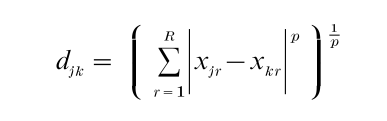
where p is generally assumed ≥ 1. The Euclidean metric, in which p = 2, is the default option in Kruskal’s (and most other) algorithm(s). Kruskal uses a well-known numerical optimization procedure called the gradient method, combined with a method of least squares monotone regression (for fitting the monotonic function f) to fit the best R-dimensional spatial representation by minimizing a measure of ‘badness of fit’ called STRESS, defined (in its original, and most widely used form) as:

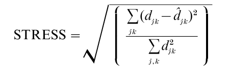
where the summations are over all values of j and k for which data are provided (so that, unlike ‘classical’ MDS, Kruskal’s algorithm easily handles missing data). More generally a weighted generalization in which each term in the summations in both the numerator and denominator is weighted by nonnegative weights input by the user (or calculated as a function of δ_jk) can be substituted for (unweighted) STRESS.

If the user is not certain of the appropriate dimensionality, solutions may be obtained for a range of values of number of dimensions, R, and a plot of STRESS vs. dimensionality, plus criteria based on interpretability, used to choose the ‘best’ value of R. See Kruskal and Wish (1978) for further discussion, and a general overview of metric and nonmetric two- way MDS.

While Euclidean distances are most often assumed, other values of p in the Minkowski-p (or L_p) metric can be used. In practice, the only alternative value of p that has been used to any extent is p = 1. This leads to what is often called the ‘city block’ or ‘Manhattan’ metric, for which there is considerable theoretical basis, especially in the case of what Shepard and others have called ‘analyzable’ or ‘nonunitary’ (often, but not necessarily, more ‘conceptual’ than ‘perceptual’) stimuli. However, as discussed in detail by Arabie et al. (1987) it is inadvisable to use Kruskal’s algorithm (or other similar algorithms) to fit a city block model, because of a particularly severe ‘local minimum’ problem (which can also less seriously affect fitting Euclidean models—but this can be dealt with reasonably effectively by procedures described by Kruskal and Wish 1978 and elsewhere). Kruskal’s approach (and many others usually characterized as ‘nonmetric’ MDS) also allow(s) the function, f, to be linear, in which case the analysis is a metric one, assuming interval or even ratio scale data (depending on whether the linear function includes an intercept, or additive constant term, or not). Other functions are also allowed.

Other approaches to two-way metric or nonmetric MDS have been proposed by Guttman, (‘Smallest Space Analysis’), by Takane et al. (ALSCAL), Ramsay (MULTISCALE), and Heiser and de Leeuw (SMACOF). Ramsay’s MULTISCALE is a maximum likelihood approach, which is more soundly based statistically than other approaches. Winsberg and Carroll (1989) proposed a ‘quasi-nonmetric’ approach to fitting an extended Euclidean model (assuming dimensions ‘specific’ to individual stimuli in addition to common dimensions underlying all the stimuli) which is also fitted via maximum likelihood procedures.

1. Individual Differences Multidimensional Scaling

The first approach to individual differences MDS was the ‘points of view’ approach proposed by Tucker and Messick in 1963. This was followed by the now dominant approach, generally called INDSCAL (Carroll and Chang 1970), for INdividual Differences multidimensional SCALing. INDSCAL, which stands ambiguously for a model, a method, and a specific computer program implemented by Carroll and Chang, accounts for individual differences in proximity data via a model assuming a common set of stimulus/object dimensions, while assuming that different subjects (or other data sources) have different patterns of saliences or importance weights for these common dimensions. In the case of similarity judgments by human subjects, the INDSCAL model makes the quite plausible assumption that each subject has a different set of scale factors (amplifications or attenuations) applied to a set of ‘fundamental’ psychological stimulus dimensions common to all individuals. It is as if each subject has a set of ‘gain controls,’ one for each of the fundamental stimulus dimensions, and that these are differently adjusted for each subject. These different weights might be due to genetic differences, to environmental factors related to different experiential histories, or, most likely, to a combination of nature (genetics) and nurture (environment).

One strength of INDSCAL is ‘dimensional uniqueness’—the property that the (estimated) stimulus dimensions are uniquely determined by similarity judgments of subjects (based on the patterns of individual differences in proximities). Equally importantly, the saliences, or perceptual importance weights of dimensions, can provide quite useful individual differences measures for subjects.

The data for individual differences MDS generally comprise a number of symmetric proximity matrices, one for each subject (or other data source). Such data are generally designated as two-mode (e.g., stimuli and subjects) but three-way (e.g., stimuli stimuli subjects). A ‘mode’ is a specific set of entities (e.g., stimuli). The number of ‘ways’ can be thought of as the number of ‘directions’ in the data table (e.g., rows, columns, and ‘slices’ for a three-way table, where both rows and columns correspond to the stimulus mode, while ‘slices’ correspond to the subject mode). The purpose of INDSCAL analysis is, given such three-way proximity data, to solve simultaneously for the stimulus coordinates and the subject weights so as to optimize the fit of the INDSCAL model to the (transformed) proximity data.

The INDSCAL method makes metric assumptions and entails a kind of three-way generalization of the ‘classical’ method for two-way MDS. The most efficient approach for implementing this analysis is provided by a program called SINDSCAL written by Pruzansky in 1975, which improves on the Carroll and Chang INDSCAL program for fitting the INDSCAL model via the INDSCAL method, in the specific case of three-way symmetric proximity data.

2. The INDSCAL Model And Method

Let δ⁽ⁱ⁾_jk be the measure of proximity between stimuli/objects j and k for subject/source i. The INDSCAL model assumes that proximities are approximately related to generalized (weighted) Euclidean distances via a function f_i (different for each subject or source), so that:

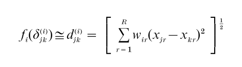
where ‘ = ’ means ‘equals, except for (unspecified) error terms.’

The INDSCAL method, most effectively implemented in Pruzansky’s SINDSCAL program, assumes f_i is linear for all i, and uses a generalization of the approach used in the ‘classical’ metric approach to two-way MDS. Where the latter uses the SVD (singular value decomposition) to derive coordinates of n stimuli on R dimensions from a single derived matrix of ‘scalar products,’ INDSCAL/SINDSCAL uses a generalization of the SVD called CANDECOMP (for CANonical DECOMPosition of N-way tables) simultaneously to fit coordinates of the R dimensions (x_jr, for j 1, 2, = n and r = 1, 2, R) for the n stimuli and weights for m (w_ir, for i = 1, 2, m and r = 1, 2, R) to a three-way array of derived scalar products. The details of the INDSCAL method for fitting the INDSCAL model are described by Carroll and Chang (1970). Other methods mentioned below for fitting the INDSCAL model make various other assumptions about the relations between proximities and weighted Euclidean distances.

In addition to accounting for individual differences among subjects or other data sources via differential patterns of weights for the R dimensions, INDSCAL has the important property—often called ‘dimensional uniqueness’—that the dimensions are—under very general conditions—uniquely oriented, and not subject to rotation. A set of necessary and sufficient conditions for this property to hold is that the subject weights are not all equal, or proportional, to one another for different subjects, for any subset of two or more dimensions.

This is true because a rotation of coordinate axes in the ‘group’ stimulus space can be shown not to yield the same set of weighted distance matrices (even if subject weights are recomputed for the rotated dimensions) as the ‘preferred’ orientation determined by the procedure fitting the INDSCAL model, so that the measure of goodness of fit to the proximity data will not be as good as for this ‘preferred’ orientation. This statistical uniqueness of INDSCAL dimensions rein-forces the fact that INDSCAL dimensions can be considered to be psychologically ‘fundamental.’ This theoretical and statistical uniqueness of INDSCAL dimensions has been supported in numerous applications in which INDSCAL dimensions, even in fairly high dimensionalities (up to nine dimensions in some cases), are almost always interpretable without rotation.

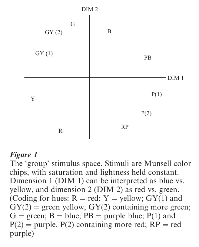
We illustrate INDSCAL by an example involving ‘points of view’ analysis of data on color perception due to Helm. In 1962 Helm and Tucker analyzed these data via this model, and found that about ten ‘points of view’ were necessary to account adequately for all the individual differences among subjects. The INDSCAL analysis accounted quite nicely for the individual differences among the 14 subjects in terms of a two dimensional solution, illustrated in Fig. 1 easily interpretable in terms of two dimensions that accord very well with physiological and psycho- physical evidence, strongly suggesting the existence of ‘blue–yellow’ and ‘red–green’ receptors. Dimension one corresponds quite well to a ‘blue vs. yellow’ (or ‘purple–blue vs. green–yellow’) dimension, and dimension two to a ‘red vs. green’ (or ‘purple–red vs. blue–green’) dimension, as can be seen in Fig.1.

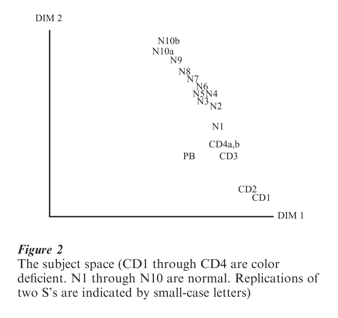
Helm included four subjects with varying degrees of red-green color deficiency, labeled (in the ‘subject space’ shown in Fig. 2) as subjects CD1 through CD4 (a and b in the last case, since the data for this subject were collected twice, about a month separating the two replications). As can be seen in Fig. 2, all the red–green color-deficient subjects had smaller weights for the red–green dimension than any of the normal subjects (coded N1 through N10 a and b). This means that the red–green dimension is less salient perceptually to the four subjects with variants of the most common types of anomalous color vision (protanomalous or deuteranomalous vision—two types of deficiency in distinguishing red from green), as would be predicted on theoretical grounds. In what is often called the ‘private perceptual space,’ constructed by applying the (square roots of the) subject weights, for each subject, as rescaling factors to the dimensions, the space for color-deficient subjects is compressed in the ‘red–green’ direction, so that for them red and green are perceived as being much closer (more similar) relatively speaking than is the case for the subjects with normal color vision.

While in one sense this INDSCAL analysis merely confirms what was learned by over a hundred years of careful physiological and psychophysical studies, had we not been aware of these studies these results might well have been helpful to scientists seeking to under- stand more fully the nature of both normal and anomalous color vision. In many other domains of study (see Wish and Carroll 1974 or Arabie et al. 1987 for examples) psychologists and other behavioral or social scientists ha e in fact learned a great deal about both the psychological (or other) dimensions, and the nature of individual differences underlying perception of important classes of stimuli (or of measured proximities of other ‘objects’).

Various alternative nonmetric and metric algorithms have been developed for fitting the INDSCAL model. Most prominent are Takane et al.’s ALSCAL (in its three-way implementation) and Ramsay’s MULTISCALE procedure, which provides methods for fitting the three-way INDSCAL model based on a maximum likelihood criterion. Carroll and Winsberg (1995) generalized their approach based on the ex- tended Euclidean model to an extended INDSCAL model, called EXSCAL, fitted by what is called a ‘quasi-nonmetric’ approach, using a maximum likelihood procedure. More recently a three-way version of SMACOF, called PROXSCAL, has been developed and is distributed by Heiser and colleagues, and has been available in SPSS, version 10 or later, since mid- 2000. This is probably the best approach for a purely nonmetric analysis of three-way proximity data in terms of the INDSCAL model.

3. Broad Definition Of Multidimensional Scaling

In its broadest definition, MDS includes a wide variety of geometric models, not only spatial distance models, for representation of psychological or other data. These can include discrete geometric models such as tree structures (often associated with hierarchical clustering), overlapping or nonoverlapping cluster structures, or more general cluster or network models. While MDS is typically associated with continuous spatial distance models for representation of proximities, the broad definition also includes other spatial models, such as what are called the vector or the unfolding/ideal point models for representation of individual differences in preference (or other dominance) data, or two-or three-way factor/components analysis models—many of which are nondistance based. For further information on MDS, in both its narrow and broader definitions, as well as for further details and/or applications of two-way and three-way MDS, see Carroll (1976, 1980), Shepard (1978), Carroll and Arabie (1980, 1998), Meulman (1992), Klauer and Carroll (1995), Carroll and Chaturvedi (1995), Carroll and Wish (1974a, 1974b), De Soete and Carroll (1992, 1996), and/or Wish and Carroll (1974).

Bibliography:

1. Arabie P, Carroll J D, DeSarbo W S 1987 Three-Way Scaling and Clustering. Sage, Newbury Park, CA
2. Carroll J D 1976 Spatial, non-spatial and hybrid models for scaling. (Presidential Address for Psychometric Society). Psychometrika 41: 439–63
3. Carroll J D 1980 Models and methods for multidimensional analysis of preferential choice (or other dominance) data. In: Lantermann E D, Feger H (eds.) Similarity and Choice. Hans Huber, Bern, Switzerland
4. Carroll J D, Arabie P 1980 Multidimensional scaling. In: Rosenzweig M R, Porter L W (eds.) Annual Review of Psychology. Annual Reviews, Palo Alto, CA
5. Carroll J D, Arabie P 1998 Multidimensional scaling. In: Birnbaum M H (ed.) Handbook of Perception and Cognition. Vol. 3: Measurement, Judgment and Decision. Academic Press, San Diego, CA
6. Carroll J D, Chang J J 1970 Analysis of individual differences in multidimensional scaling via an N-way generalization of ‘Eckart–Young’ decomposition. Psychometrika 35: 283–319
7. Carroll J D, Chaturvedi A 1995 A general approach to clustering and multidimensional scaling of two-way, three-way, or higher-way data. In: Luce R D, D’Zmura M, Hoffman D D, Iverson G, Romney A K (eds.) Geometric Representations of Perceptual Phenomena. Erlbaum, Mahwah, NJ
8. Carroll J D, Wish M 1974a Models and methods for three-way multidimensional scaling. In: Krantz D H, Atkinson R C, Luce R D, Suppes P (eds.) Contemporary Developments in Mathematical Psychology. W H Freeman, San Francisco, CA, Vol. 2
9. Carroll J D, Wish M 1974b Multidimensional perceptual models and measurement methods. In: Carterette E C, Friedman M P (eds.) Handbook of Perception. Academic Press, New York, Vol. 2
10. Coombs C H 1964 A Theory of Data. Wiley, New York
11. De Soete G, Carroll J D 1992 Probabilistic multidimensional models of pairwise choice data. In: Ashby F G (ed.) Multidimensional Models of Perception and Cognition. Erlbaum, Hillsdale, NJ
12. De Soete G, Carroll J D 1996 Tree and other network models for representing proximity data. In: Arabie P, Hubert L J, De Soete G (eds.) Clustering and Classification. World Scientific, River Edge, NJ
13. Klauer K C, Carroll J D 1995 Network models for scaling proximity data. In: Luce R D, D’Zmura M, Hoffman D D, Iverson G, Romney A K (eds.) Geometric Representations of Perceptual Phenomena. Erlbaum, Mahwah, NJ
14. Kruskal J B, Wish M 1978 Multidimensional Scaling. Sage, Beverly Hills, CA
15. Meulman J J 1992 The integration of multidimensional scaling and multivariate analysis with optimal transformations. Psychometrika 57: 539–65
16. Shepard R N 1978 The circumplex and related topological manifolds in the study of perception. In: Shye S (ed.) Theory Construction and Data Analysis in the Behavioral Science 1st edn.. Jossey-Bass, San Francisco, CA
17. Torgerson W S 1958 Theory and Methods of Scaling. Wiley, New York
18. Wish M, Carroll J D 1974 Applications of individual differences scaling to studies of human perception and judgment. In: Carterette E C, Friedman M P (eds.) Handbook of Perception: Psychophysical Judgment and Measurement. Academic Press, New York