Univariate Methods of Exploratory Data Analysis Research Paper

Other efforts, parallel to Tukey’s, led to alternative, and generally more complex, exploratory methods. The leading examples are correspondence analysis, developed by Benzecri and the French school; multivariate scaling methods; and semi-parametric approaches to prediction and classification.

1. Main Themes Of EDA

At the core of the EDA approach lie four main themes: display, re-expression, resistance and residuals.

(a) Displays (most of them graphical) allow the analyst to see the behavior of the data and, as analysis proceeds, the behavior of residuals and various diagnostic measures. EDA emphasizes the frequent use of displays, to ensure that unexpected features are not overlooked. The most common displays include the stem-and-leaf display, the boxplot, scatterplots of residuals, and the spread-vs.-level plot.

(b) Re-expression involves applying a single mathematical transformation (such as the square root or the logarithm) to each data value. The aim is to simplify, and thus make more effective, the analysis of the data. Depending on the structure of the data, the simplification may come from promoting symmetry, constancy of variability, straightness of relationship, or additivity of effect. EDA asks, at nearly the first opportunity, whether the scale in which the data are presented is satisfactory. If not, it freely tries a likely transformation.

The re-expressions most often used in EDA come from the family of functions known as power trans-formations, which take y into y^p (almost always with a simple value of p such as 1/2, -1, or 2), together with the logarithm (which, for data analysis purposes, fits into the power family at p 0) . For example, in a study of the levels of nicotine in the blood and urine of smokers and nonsmokers, the analysis gained simplicity by reexpressing the nicotine concentrations in the logarithmic scale.

(c) Resistance provides insensitivity to misbehavior or unusual behavior in data. An analysis or summary is resistant if an arbitrary change in any small part of the data produces only a small change in the analysis or summary. EDA emphasizes resistance because experience suggests that ‘good’ data seldom contain less than about 5 percent gross errors.

The notion of robustness is akin to resistance, but not the same. Robustness generally implies insensitivity to departures from assumptions surrounding an underlying probabilistic model. (Resistance is sometimes mentioned as one aspect of ‘qualitative robustness.’)

In summarizing the location of a sample, the median is highly resistant. (In terms of efficiency, it is not so highly robust because other estimators achieve greater efficiency across a broader range of distributions.) By contrast, the mean is highly nonresistant. A number of exploratory techniques for more structured forms of data provide resistance because they are based on the median.

(d) Residuals are what remain of data after a summary or fitted model has been subtracted out, according to the schematic equation

For example, if the data are the pairs (x_i, y_i) and the fit is the line y_i =a +bx_i, then the residuals are r_i=y_i-y_i.

EDA regards a careful examination of the residuals as an essential step in analyzing a set of data. This emphasis reflects the tendency of resistant analyses to provide a clear separation between dominant behavior and unusual behavior in the data. When the bulk of the data follows a consistent pattern, that pattern determines a resistant fit. The residuals then contain any drastic departures from the pattern, as well as the customary chance fluctuations. Unusual residuals suggest a need to check on the circumstances surrounding those observations. As in more traditional practice, the residuals can warn of systematic difficulties with the data—curvature, non-additivity, and non-constancy of variability.

The examples and discussion that follow illustrate displays (via stem-and-leaf displays and boxplots), resistance (median polish), residuals, and re-expression.

2. Example 1: Stem-And-Leaf Displays (Florida Voting)

The initial results of the 2000 US presidential election focused intense attention on the state of Florida, where the difference in total votes cast for George W. Bush and Albert Gore was so small that state law required a recount and thus delayed the outcome. Among the unusual features of the Florida voting was the relatively large number of votes cast in Palm Beach County for Patrick Buchanan, the candidate of the Reform Party (3407 out of 430,762 votes). Critics argued that most of those votes had been intended for Gore, but were recorded for Buchanan because of a problem with the type of ballot.

A number of analyses compared the results in Palm Beach County against those in other counties. Without explaining the reasons for those choices, one analyst selected the data from the 30 counties in which Bush received more than 30,000 votes and calculated the ratio of the number of Buchanan votes to the number of Bush votes, concluding that the probability of the ratio in Palm Beach County by pure chance was extremely small.

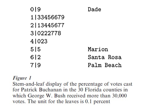
For those 30 counties Fig. 1 shows a stem-and-leaf display of the percentage of votes for Buchanan (out of the total number of votes for four candidates: Bush, Gore, Buchanan, and Ralph Nader). In overall outline this display resembles a histogram with an interval width of 0.1 percent, but it shows more detail of the data values by using the 0.01 percent digit of each percentage instead of merely enclosing a uniform amount of area. This feature makes it easy to go back from a part of the display to the individual data values (and their identities) in the listing of the data—a valuable step in EDA.

Several alternatives and refinements permit the stem-and-leaf display to accommodate a wide variety of data patterns. The interval width (that is, the range of data values represented by one line in the display) may be 2, 5, or 10 times a power of 10; and stray observations may be listed separately at each end so as not to distort the scale. The use of positive and negative stems readily handles sets of residuals.

In Fig. 1 Palm Beach County’s 0.79 percent for Buchanan is noticeably high (indeed, another EDA technique would flag it as ‘outside’ and hence deserving investigation). But the 0.55 percent for Marion County and the 0.62 percent for Santa Rosa County are also noticeable at the high end. The layout of the stem-and-leaf display makes it easy to include tags that identify a few data values at either end.

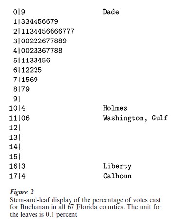
The analyst’s choice of counties with more than 30,000 votes for Bush naturally raises a question about the extent of support for Buchanan in the other 37 counties of Florida. Figure 2 shows a stem-and-leaf display for all 67 counties. In the context of the whole state, Palm Beach County no longer stands out; seven counties had a percentage for Buchanan higher than 0.79 percent, and two of those were above 1.6 percent. Those seven counties, however, are small; most cast fewer than 8,000 total votes for the four candidates. Also, geographically, they are all located in north Florida, far from Palm Beach County. Thus, among counties with larger numbers of voters, it still appears that Palm Beach County produced an unusually large percentage for Buchanan. A stem-and-leaf display of the vote totals (not shown) reveals a clear gap around 40,000. Modifying Fig. 1 to include all counties with totals greater than 40,000 would add three counties, whose percentages for Buchanan were 0.21 percent, 0.26 percent, and 0.47 percent.

Even after this modification the position of Palm Beach County in Fig. 1 does not form the basis for a conclusion. It does invite further examination. Other analysts responded, taking into account the voting in counties throughout the US, precinct-level voting in Palm Beach County, and voting in other Florida elections. For example, even if one uses only data from Florida counties, a scatterplot of the percentage for Buchanan against the percentage of Bush (or against the percentage of Gore) shows that Palm Beach County is very far from the other counties.

3. Example 2: Boxplots (Childhood Immunization)

In the United States the Centers for Disease Control and Prevention use the National Immunization Survey (NIS) to monitor the extent to which children 19 to 35 months of age have received the recommended vaccinations. A telephone survey, the NIS uses randomdigit dialing to locate households that contain such children, in each of 78 Immunization Action Plan (IAP) areas that cover the US. It interviews the children’s parents or guardians, and also (by mail) contacts the children’s vaccination providers to obtain data from the child’s medical record. In a year the NIS completes household interviews for approximately 400 children in each IAP area, and it obtains provider data for about two-thirds of them.

For each IAP area, each state, and the whole US, the NIS produces estimates of vaccination coverage (the percentage of children who are up-to-date) for several individual vaccinations and for selected series of shots, such as the 4:3:1 series (4 or more doses of diphtheria and tetanus toxoids and pertussis vaccine, 3 or more doses of poliovirus vaccine, and 1 or more doses of measles-containing vaccine), which the CDC has used in allocating funds to states.

The CDC selected the 28 urban IAP areas for a variety of reasons, including concern for lower rates of vaccination coverage. For one overall comparison, Fig. 3 shows parallel boxplots of the estimates of 4:3:1 coverage in 1997 for the 50 states and the 28 urban areas.

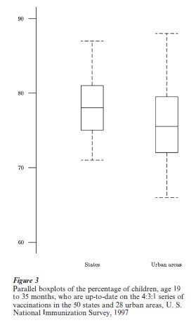
In a boxplot (also called a ‘schematic plot’) the box extends from the lower hinge (an approximate quartile) to the upper hinge and has a line across it at the median. The dashed lines show the extent of the data, except for observations that are likely strays (defined according to a rule based on the hinges). Such strays (when present) appear individually, in order to focus attention on them. The general intent is to indicate the median, outline the middle half of the data, and show the range, with more detail at the ends if needed.

The message of Fig. 3 is that 4:3:1 vaccination coverage is typically lower in the urban areas than in the states—by about 2 percentage points according to the hinges and median. But the range is greater in the urban IAP areas, from 66 percent in Houston and 67 percent in El Paso, Texas to 88 percent in Boston, Massachusetts.

4. Example 3: Median Polish, Residuals (Hotel Occupancy)

In 1983, as several new hotels were under construction in Boston, operators of existing major hotels were concerned about the impact on their business. Table 1 shows the occupancy rates for 11 major Metropolitan Boston hotels, month by month, for January through June 1983. One approach to exploring such a two-way table uses an additive fit of the form

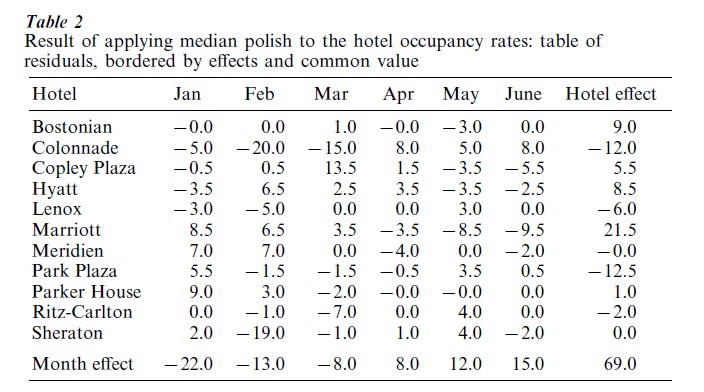
with a row effect, a_i, for each hotel and a column effect, b_j, for each month. The EDA technique known as median polish arrives at such a fit by iteratively subtracting row medians and column medians, first from the table of data and then from the table left by the previous iteration. The common value, m, is determined by centering the effects so that the median of the a_i is 0 and the median of the b_j is 0. The use of the median gives the fit resistance: isolated behavior of the data in a few cells of the table will tend to have only a minor impact on the fit.

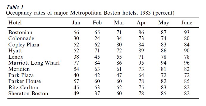
For the hotel occupancy rates Table 2 shows the two-way table of residuals, y_ij -y_ij, bordered by the hotel effects, the month effects, and the common value. The month effects (ranging from -22.0 to +15.0) show occupancy rates in Boston hotels increasing substantially from January to June. Among the hotel effects the Marriott Long Wharf (at 21.5) stands out as having higher occupancy than the other hotels, and the Colonnade and the Park Plaza (at -12.0 and + 12.5, respectively) were substantially lower. A stem and-leaf display of the residuals (not shown) calls attention to three sizable negative residuals ( -20.0, -19.0, and -15.0) and one sizable positive residual (+13.5). These indicate that the Colonnade (beyond its generally low occupancy) had unusually low occupancy in February and March, that the Sheraton Boston had unusually low occupancy in February, and that the Copley Plaza had unusually high occupancy in March.

5. Example 4: Everyday Re-Expressions

In a number of applications from a variety of fields, a re-expression has become so customary that no one mentions it. By the time the data or results are presented, they are already in the transformed scale. Examples include established relationships in science and engineering, as well as contemporary data (see also Hoaglin 1988).

For earthquakes the Richter scale expresses the strength in logarithmic units (base 10). The magnitude is defined as the logarithm of the amplitude recorded by a particular type of seismograph (at a specified distance from the epicenter).

In measuring the intensity of sounds, the decibel scale is logarithmically related to sound pressure.

Measurements of the fuel consumption of automobiles often involve determining the number of gallons of gasoline that a car used on a standard test course. Thus, the ratings in miles per gallon are the result of a reciprocal transformation.

6. Literature

The first published presentation of exploratory data analysis was the preliminary edition (1970–71) of the book by John W. Tukey, whose 1977 edition represents the definitive account of the subject. Mosteller and Tukey (1977) also includes substantial discussion of exploratory attitudes and techniques.

The two volumes of the Statistician’s Guide to Exploratory Data Analysis (Hoaglin et al. 1983, 1985) discuss the rationale and development of a number of EDA techniques, explain and illustrate connections with classical statistical theory, and introduce new techniques.

Hoaglin et al. (1991) extend the basic attitudes and techniques of EDA to factorial analysis of variance.

Broader discussions of the roles of exploratory and confirmatory data analysis in scientific inquiry appear in Tukey (1972) and Tukey (1980).

Bibliography:

1. Hoaglin D C 1988 Transformations in everyday experience. CHANCE 1, 4: 40–5
2. Hoaglin D C, Mosteller F, Tukey J W 1983 Understanding Robust and Exploratory Data Analysis, Wiley Classics Library edition 2000. Wiley, New York
3. Hoaglin D C, Mosteller F, Tukey J W 1985 Exploring Data Tables, Trends, and Shapes. Wiley, New York
4. Hoaglin D C, Mosteller F, Tukey J W 1991 Fundamentals of Exploratory Analysis of Variance. Wiley, New York
5. Mosteller F, Tukey J W 1977 Data Analysis and Regression: A Second Course in Statistics. Addison-Wesley, Reading, MA
6. Tukey J W 1970–71 Exploratory Data Analysis, limited preliminary edition. Addison-Wesley, Reading, MA [available from University Microfilms]
7. Tukey J W 1972 Data analysis, computation, and mathematics. Quarterly of Applied Mathematics 30: 51–65
8. Tukey J W 1977 Exploratory Data Analysis. Addison-Wesley, Reading, MA
9. Tukey J W 1980 We need both exploratory and confirmatory. The American Statistician 34: 23–5