Missing Statistical Data Research Paper

(a) In longitudinal studies, data are missing because of attrition, i.e., subjects drop out prior to the end of the study.

(b) In most surveys, some individuals provide no information because of noncontact or refusal to respond (unit nonresponse). Other individuals are contacted and provide some information, but fail to answer some of the questions (item nonresponse). See Sample Surveys: The Field.

(c) Information about a variable is partially recorded. A common example in social science is right censoring, where times to an event (death, finding a job) are recorded, and for some individuals the event has still not taken place when the study is terminated. The times for these subjects are known to be greater that corresponding to the latest time of observation, but the actual time is unknown. Another example of partial information is inter al censoring, where it is known that the time to an event lies in an interval. For example in a longitudinal study of employment, it may be established that the event of finding a job took place some time between two interviews.

(d) Often indices are constructed by summing values of particular items. For example, in economic studies, total net worth is a combination of values of individual assets or liabilities, some of which may be missing. If any of the items that form the index are missing, some procedure is needed to deal with the missing data.

(e) Missing data can arise by design. For example, suppose one objective in a study of obesity is to estimate the distribution of a measure Y₁ of body fat in the population, and correlate it with other factors. Suppose Y₁ is expensive to measure but a proxy measure Y₂, such as body mass index, which is a function of height and weight, is inexpensive to measure. Then it may be useful to measure Y₂ and covariates, X, for a large sample but Y₁, Y₂ and X for a smaller subsample. The subsample allows predictions of the missing values of Y₁ to be generated for the larger sample, yielding more efficient estimates than are possible from the subsample alone.

Unless missing data are deliberately incorporated by design (such as in (e)), the most important step in dealing with missing data is to try to avoid it during the data-collection stage. Because data are likely to be missing in any case, however, it is important to try to collect covariates that are predictive of the missing values, so that an adequate adjustment can be made. In addition, the process that leads to missing values should be determined during the collection of data if possible, since this information helps to model the missing-data mechanism when an adjustment for the missing values is performed (Little 1995).

Three major approaches to the analysis of missing data can be distinguished:

(a) discard incomplete cases and analyze the remainder (complete-case analysis), as discussed in Sect. 3;

(b) impute or fill in the missing values and then analyze the filled-in data, as discussed in Sect. 4; and

(c) analyze the incomplete data by a method that does not require a complete (that is, a rectangular) data set.

With regard to (c), we focus in Sects. 6, 7, and 8 on powerful likelihood-based methods, specifically maxi- mum likelihood (ML) and Bayesian simulation. See Bayesian Statistics. The latter is closely related to multiple imputation (Rubin 1987, 1996), an extension of single imputation that allows uncertainty in the imputations to be reflected appropriately in the analysis, as discussed in Sect. 5.

A basic assumption in all our methods is that missingness of a particular value hides a true underlying value that is meaningful for analysis. This may seem obvious but is not always the case. For example, consider a longitudinal analysis of employment; for subjects who leave the study because they move to a different location, it makes sense to consider employment history after relocation as missing, whereas for subjects who die during the course of the study, it is clearly not reasonable to consider employment history after time of death as missing; rather it is preferable to restrict the analysis of employment to individuals who are alive. A more complex missing data problem arises when individuals leave a study for unknown reasons, which may include relocation or death.

Because the problem of missing data is so pervasive in the social and behavioral sciences, it is very important that researchers be aware of the availability of principled approaches that address the problem. Here we overview common approaches, which have quite limited success, as well as principled approaches, which generally address the problem with substantial success.

2. Pattern And Mechanism Of Missing Data

The pattern of the missing data simply indicates which values in the data set are observed and which are missing. Specifically, let Y= ( y_ij) denote an (n × p ) rectangular dataset without missing values, with ith row y_i = ( y_i , …, y_ip) where y_ij is the value of variable Y_j for subject i. With missing values, the pattern of missing data is defined by the missing-data indicator matrix M = ( m_ij ), such that m_ij = 1 if y_ij is missing and m_ij = 0 if y_ij is present.

Some methods for handling missing data apply to any pattern of missing data, whereas other methods assume a special pattern. An important example of a special pattern is univariate nonresponse, where miss-ingness is confined to a single variable. Another is monotone missing data, where the variables can be arranged so that Y_j+1, …, Y_p are missing for all cases where Y_j is missing, for all j = 1, …, p – 1. The result is a ‘staircase’ pattern, where all variables and units to the left of the broken line forming the staircase are observed, and all to the right are missing. This pattern arises commonly in longitudinal data subject to attrition, where once a subject drops out, no more subsequent data are observed.

The missing-data mechanism addresses the reasons why values are missing, and in particular whether these reasons relate to values in the data set. For example, subjects in a longitudinal intervention may be more likely to drop out of a study because they feel the treatment was ineffective, which might be related to a poor value of an outcome measure. Rubin (1976) treated M as a random matrix, and characterized the missing-data mechanism by the conditional distribution of M given Y, say f ( M|Y, φ), where φ denotes unknown parameters. When missingness does not depend on the values of the data Y, missing or observed, that is, f ( M|Y, φ) = f ( M|φ) for all Y, φ, the data are called missing completely at random (MCAR). MCAR does not mean that the pattern itself is random, but rather that missingness does not depend on the data values. An MCAR mechanism is plausible in planned missing-data designs as in example (e) above, but is a strong assumption when missing data do not occur by design, because missingness often does depend on recorded variables.

Let Y_obs denote the observed values of Y and Y_mis the missing values. A less restrictive assumption is that missingness depends only on values Y_obs that are observed, and not on values Y_mis that are missing. That is:

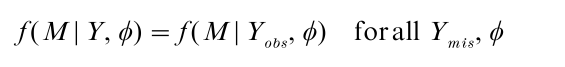
The missing data mechanism is then called missing at random (MAR). Many methods for handling missing data assume the mechanism is MCAR, and yield biased estimates when the data are not MCAR. Better methods rely only on the MAR assumption.

3. Complete-Case, Available-Case, And Weighting Analysis

A common and simple method is complete-case (CC) analysis, also known as listwise deletion, where incomplete cases are discarded and standard analysis methods applied to the complete cases. In many statistical packages this is the default analysis. Valid (but often suboptimal) inferences are obtained when the missing data are MCAR, since then the complete cases are a random subsample of the original sample with respect to all variables. However, complete-case analysis can result in the loss of a substantial amount of information available in the incomplete cases, particularly if the number of variables is large.

A serious problem with dropping incomplete cases is that the complete cases are often easily seen to be a biased sample, that is, the missing data are not MCAR. The size of the resulting bias depends on the degree of deviation from MCAR, the amount of missing data, and the specifics of the analysis. In sample surveys this motivates strenuous attempts to limit unit nonresponse though multiple follow-ups, and surveys with high rates of unit nonresponse (say 30 percent or more) are often considered unreliable for making inferences to the whole population.

A modification of CC analysis, commonly used to handle unit nonresponse in surveys, is to weight respondents by the inverse of an estimate of the probability of response. A simple approach is to form adjustment cells (or subclasses) based on background variables measured for respondents and nonrespondents; for unit nonresponse adjustment, these are often based on geographical areas or groupings of similar areas based on aggregate socioeconomic data. All nonrespondents are given zero weight and the nonresponse weight for all respondents in an adjustment cell is then the inverse of the response rate in that cell. This method removes the component of nonresponse bias attributable to differential nonresponse rates across the adjustment cells, and eliminates bias if within each adjustment cell respondents can be regarded as a random subsample of the original sample within that cell (i.e., the data are MAR given indicators for the adjustment cells).

With more extensive background information, a useful alternative approach is response propensity stratification, where (a) the indicator for unit nonresponse is regressed on the background variables, using the combined data for respondents and nonrespondents and a method such as logistic regression appropriate for a binary outcome; (b) a predicted response probability is computed for each respondent based on the regression in (a); and (c) adjustment cells are formed based on a categorized version of the predicted response probability. Theory (Rosenbaum and Rubin 1983) suggests that this is an effective method for removing nonresponse bias attributable to the background variables when unit nonresponse is MAR.

Although weighting methods can be useful for reducing nonresponse bias, they do have serious limitations. First, information in the incomplete cases is still discarded, so the method is inefficient. Weighted estimates can have unacceptably high variance, as when outlying values of a variable are given large weights. Second, variance estimation for weighted estimates with estimated weights is problematic. See Estimation: Point and Inter al. Explicit formulas are available for simple estimators such as means under simple random sampling (Oh and Scheuren 1983), but methods are not well developed for more complex problems, and often ignore the component of variability arising from estimating the weight from the data.

Available-case (AC) analysis (Little and Rubin 1987 Sect. 3.3) is a straightforward attempt to exploit the incomplete information by using all the cases available to estimate each individual parameter. For example, suppose the objective is to estimate the correlation matrix of a set of continuous variables Y₁, …, Y_p. See Multivariate Analysis: Overview. Complete-case analysis uses the set of complete cases to estimate all the correlations; AC analysis uses all the cases with both Y_j and Y_k observed to estimate the correlation of _Yj and Y_k,1 ≤ j, k ≤ p. Since the sample base of available cases for measuring each correlation includes at least the set of complete cases, the AC method appears to make better use of available information. The sample base changes from correlation to correlation, however, creating potential problems when the missing data are not MCAR or variables are highly correlated. In the presence of high correlations, there is no guarantee that the AC correlation matrix is even positive definite. Haitovsky’s (1968) simulations concerning regression with highly correlated continuous data found AC markedly inferior to CC. On the other hand, Kim and Curry (1977) found AC superior to CC in simulations based on weakly correlated data. Simulation studies comparing AC regression estimates with maximum likelihood (ML) under normality (Sect. 6) suggest that ML is superior even when underlying normality assumptions are moderately violated (Little 1988a). Although AC estimates are easy to compute, standard errors are more complex. The method cannot be generally recommended, even under the restrictive MCAR.

4. Single Imputation

Methods that impute or fill in the missing values have the advantage that, unlike CC analysis, observed values in the incomplete cases are retained. A simple version of the method imputes missing values by their unconditional sample means based on the observed data. This method can yield satisfactory point estimates of means and totals, but it yields inconsistent estimates of other parameters such as variances, covariance matrices or regression coefficients, and it overstates precision (Little and Rubin 1987, Chap. 3). Thus it cannot be recommended in any generality.

An improvement is conditional mean imputation, in which each missing value is replaced by an estimate of its conditional mean given the values of observed values. For example, in the case of univariate nonresponse with Y₁, …, Y_p−1 fully observed and Y_p sometimes missing, one approach is to classify cases into cells based on similar values of observed variables, and then to impute missing values of Y_p by the within-cell mean from the complete cases in that cell. A more general approach is regression imputation, in which the regression of Y_p on Y₁, …, Y_p−1 is estimated from the complete cases, and the resulting prediction equation is used to impute the estimated conditional mean for each missing value of Y_p. For a general pattern of missing data, the missing values for each case can be imputed from the regression of the missing variables on the observed variables, computed using the set of complete cases. Iterative versions of this method lead (with some important adjustments) to ML estimates under multivariate normality (Little and Rubin 1987, Chap. 8).

Although conditional mean imputation incorporates information from the observed variables and yields best predictions of the missing values in the sense of mean squared error, it leads to distorted estimates of quantities that are not linear in the data, such as percentiles, correlations and other measures of association, as well as variances and other measures of variability. A solution to this problem of point estimation is to use random draws rather than best predictions to preserve the distribution of variables in the filled-in data set. An example is stochastic regression imputation, in which each missing value is replaced by its regression prediction plus a random error with variance equal to the estimated residual variance.

Hot-deck methods impute actual values observed in the dataset. An example is the Current Population Survey (CPS) hot deck for imputing income items in that survey. For each nonrespondent on one or more income items, the CPS hot-deck finds a matching respondent based on variables that are observed for both; the missing income items for the nonrespondent are then replaced by the respondent’s values. When no match can be found for a nonrespondent based on all of the variables, the algorithm searches for a match at a lower level of detail, obtained by omitting some variables and collapsing the categories of others. A more general approach to hot-deck imputation matches nonrespondents and respondents using a distance function based on the observed variables. For example, predicti e mean matching (Little 1988b) that have similar predictive means from a regression of the missing variable on observed variables. This method is somewhat robust to misspecification of the regression model used to create the matching metric.

The imputation methods discussed so far assume the missing data are MAR. In contrast, models that are not missing at random (NMAR) assert that even if a respondent and nonrespondent to Y_p appear identical with respect to observed variables Y₁, …, Y_p−1, their Y_p-values differ systematically. Lillard et al. (1986), for example, discussed NMAR imputation models for missing CPS data. It is also possible to create a NMAR hot-deck procedure; for example, respondents’ values that are to be imputed to nonrespondents could be multiplied by an inflation or deflation factor that depends on the variables that are observed. A crucial point about the use of NMAR models is that there is never direct evidence in the data to address the validity of their underlying assumptions. Thus, whenever NMAR models are being considered, it is prudent to consider several NMAR models and explore the sensitivity of analyses to the choice of model (Rubin 1977, Little and Wang 1996).

5. Multiple Imputation

A serious defect with imputation is that it invents data. A single imputed value cannot represent the uncertainty about which value to impute, so analyses that treat imputed values just like observed values generally underestimate uncertainty, even if nonresponse is modeled correctly and randomly drawn imputations are created. Large-sample results show that for simple situations with 30 percent of the information missing, single imputation under the correct model results in nominal 90 percent confidence intervals having actual coverages below 80 percent. The inaccuracy of nominal levels is even more extreme in multiparameter testing problems (Rubin 1987, Chap. 4).

A modification of imputation that fixes this problem is multiple imputation (MI) (Rubin 1987). Instead of imputing a single set of draws for the missing values, a set of M (say M = 5) datasets are created, each containing different sets of draws of the missing values from their joint predictive distribution. We then apply the standard complete-data analysis to each of the M datasets and combine the results in a simple way. In particular for scalar estimands, the MI estimate is the average of the estimates from the M datasets, and the variance of the estimate is the average of the variances from the five datasets plus 1 + 1/M times the sample variance of the estimates over the M datasets (The factor 1 + 1/M is a small-M correction). The last quantity here estimates the contribution to the variance from imputation uncertainty, missed (i.e., set to zero) by single imputation methods. Another benefit of multiple imputation is that the averaging over datasets results in more efficient point estimates than does single random imputation. Often MI is not much more difficult than doing a single imputation—the additional computing from repeating an analysis M times is not a major burden, and methods for combining inferences are straightforward. Most of the work involves generating good predictive distributions for the missing values, which is needed for consistent point estimation in any case. A more detailed discussion of multiple imputation appears elsewhere in this encyclopedia.

6. Maximum Likelihood For Ignorable Models

There are statistical methods that allows the analysis a nonrectangular dataset without having to impute the missing values. In particular, maximum likelihood (ML) avoids imputation by formulating a statistical model and basing inference on the likelihood function of the incomplete data. Define Y and M as above, and let X denote an ( n × q) matrix of fixed covariates, assumed fully observed, with ith row x_i = ( x_i1, …, x_iq ) where x_ij is the value of covariate X_j for subject i. Covariates that are not fully observed should be treated as random variables and modeled with the set of Y_j’s (Little and Rubin 1987 Chap. 5). The data and missing-data mechanism are modeled in terms of a joint distribution for Y and M given X. Selection models specify this distribution as:

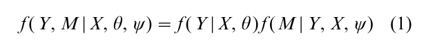
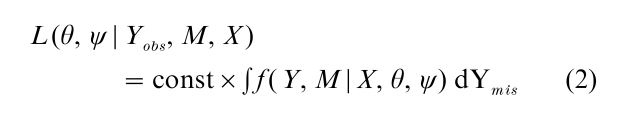
where f ( Y|X, θ ) is the model in the absence of missing values, f ( M|Y, X, ψ ) is the model for the missing- data mechanism, and θ and ψ are unknown parameters. The likelihood of θ, ψ given the data Y_obs, M, X is then proportional to the density of Y_obs, M given X regarded as a function of the parameters θ, ψ, and this is obtained by integrating out the missing data Y_mis from Eqn. (1), that is:

The likelihood of θ ignoring the missing-data mechanism is obtained by integrating the missing data from the marginal distribution of Y given X, that is:

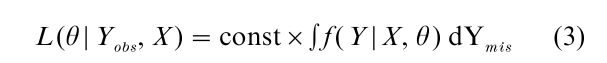
The likelihood (3) is easier to work with than (2) since it is easier to handle computationally; more important, avoids the need to specify a model for the missing-data mechanism, about which little is known in many situations. Hence it is important to determine when valid likelihood inferences are obtained from (3) instead of the full likelihood (2). Rubin (1976) showed that valid inferences about θ are obtained from (3) when the data are MAR, that is:

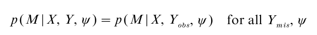
If in addition θ and ψ are distinct in the sense that they have disjoint sample spaces, then likelihood inferences about θ based on (3) are equivalent to inferences based on (2); the missing-data mechanism is then called ignorable for likelihood inferences. Large-sample inferences about θ based on an ignorable model are based on ML theory, which states that under regularity conditions

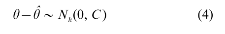
where θ is the value of θ that maximizes (3), and N_k(0, C ) is the k-variate normal distribution with mean zero and covariance matrix C, given by the inverse of an information matrix; for example C = I⁻¹ (θ) where I is the observed information matrix I (θ) = – ϐ²log L (θ|Y_obs, X ) / ϐθϐθ^T, or C = J⁻¹ (θ) where J (θ ) is the expected value of I (θ ). As in (Little and Rubin 1987), Eqn. (4) is written to be open to a frequentist interpretation if θ is regarded as random and θ fixed, or a Bayesian interpretation if θ is regarded as random and θ fixed. Thus if the data are MAR, the likelihood approach reduces to developing a suitable model for the data and computing θ and C.

In many problems maximization of the likelihood to compute θ requires numerical methods. Standard optimization methods such as Newton-Raphson or Scoring can be applied. Alternatively, the Expectation- Maximization (EM) algorithm (Dempster et al. 1977) can be applied, a general algorithm for incomplete data problems that provides an interesting link with imputation methods. The history of EM, which dates back to the beginning of this century for particular problems, is sketched in Little and Rubin (1987) and McLachlan and Krishnan (1997).

7. The EM Algorithm For Ignorable Models

For ignorable models, let L (θ|Y_obs, Y_mis, X ) denotes the likelihood of θ based on the hypothetical complete data Y = ( Y_obs, Y_mis) and covariates X. Let θ^(t) denote an estimate of θ at iteration t of EM. Iteration t + 1 consists of an E-step and M-step. The E-step computes the expectation of log L (θ|Y_obs, Y_mis, X ) over the conditional distribution of Y_mis given Y_obs and X, evaluated at θ = θ^(t), that is, Q (θ|θ^(t)) = ∫ log L (θ|Y_obs ,Y_mis, X ) f (Y_mis|Y_obs, X, θ^(t)) dY_mis. When the complete data belong to an exponential family with complete-data sufficient statistics S, the E-step simplifies to computing expected values of these statistics given the observed data and θ = θ^(t), thus in a sense ‘imputing’ the sufficient statistics. The M-step determines θ^(t+1) to maximize Q (θ|θ^(t)) with respect to θ. In exponential family cases, this step is the same as for complete data, except that the complete-data sufficient statistics S are replaced by their estimates from the Estep. Thus the M-step is often easy or available with existing software, and the programming work is mainly confined to E-step computations. Under very general conditions, each iteration of EM strictly increases the loglikelihood, and under more restrictive but still general conditions, EM converges to a maximum of the likelihood function. If a unique finite ML estimate of θ exists, EM will find it.

Little and Rubin (1987) provided many applications of EM to particular models, including: multivariate normal data with a general pattern of missing values and the related problem of multivariate linear regression with missing data; robust inference based on multivariate t models; loglinear models for multiway contingency tables with missing data; and the general location model for mixtures of continuous and categorical variables, which yields ML algorithms for logistic regression with missing covariates. An extensive Bibliography: of the myriad of EM applications is given in Meng and Pedlow (1992).

The EM algorithm is reliable but has a linear convergence rate determined by the fraction of missing information. Extensions of EM (McLachlan and Krishnan 1997) can have much faster convergence: ECM, ECME, AECM, and PX-EM (Liu et al. 1998). EM-type algorithms are particularly attractive in problems where the number of parameters is large. Asymptotic standard errors based on bootstrap methods (Efron 1994) are also available, at least in simpler situations. An attractive alternative is to switch to a Bayesian simulation method that simulates the posterior distribution of θ (see Sect. 9).

8. Maximum Likelihood For Nonignorable Models

Nonignorable, non-MAR models apply when missingness depends on the missing values (see Sect. 2). A correct likelihood analysis must be based on the full likelihood from a model for the joint distribution of Y and M. The standard likelihood asymptotics apply to nonignorable models providing the parameters are identified, and computational tools such as EM, also apply to this more general class of models. However, often information to estimate both the parameters of the missing-data mechanism and the parameters of the complete-data model is very limited, and estimates are sensitive to misspecification of the model. Often a sensitivity analysis is needed to see how much the answers change for various assumptions about the missing-data mechanism.

There are two broad classes of models for the joint distribution of Y and M. Selection models model the joint distribution as in Eqn. (1). Pattern-mixture models specify:

where φ and π are unknown parameters, and now the distribution of Y is conditioned on the missing-data pattern M (Little 1993). Equations (1) and (5) are simply two different ways of factoring the joint distribution of Y and M. When M is independent of Y, the two specifications are equivalent with θ = φ and ψ = π. Otherwise (1) and (5) generally yield different models. Rubin (1977) and Little (1993) also consider pattern-set mixture models, a more general class of models that includes pattern-mixture and selection models as special cases.

Although most of the literature on missing data has concerned selection models of the form (1) for univariate nonresponse, pattern-mixture models seem more natural when missingness defines a distinct stratum of the population of intrinsic interest, such as individuals reporting ‘don’t know’ in an opinion survey. However, pattern-mixture models can also provide inferences for parameters θ of the complete-data distribution, by expressing the parameters of interest as functions of the pattern-mixture model parameters φ and π. An advantage of the pattern-mixture modeling approach over selection models is that assumptions about the form of the missing-data mechanism are sometimes less specific in their parametric form, since they are incorporated in the model via parameter restrictions. This idea is explained in specific normal models in Little and Wang (1996), for example.

Heitjan and Rubin (1991) extended the formulation of missing-data problems via the joint distribution of Y and M to more general incomplete data problems involving coarsened data. The idea is replace the binary missing-data indicators by coarsening variables that map the y_ij values to coarsened versions z_ij( y_ij). Full and ignorable likelihoods can be defined for this more general setting. This theory provides a bridge between missing-data theory and theories of censoring in the survival analysis literature. The EM algorithm can be applied to ignorable models by including the missing data (or coarsening) indicator in the complete-data likelihood.

9. Bayesian Simulation Methods

Maximum likelihood is most useful when sample sizes are large, since then the log-likelihood is nearly quadratic and can be summarized well using the ML estimate of θ and its large sample variance-covariance matrix. When sample sizes are small, a useful alternative approach is to add a prior distribution for the parameters and compute the posterior distribution of the parameters of interest. For ignorable models this is

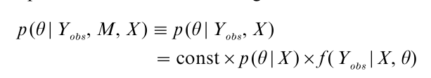
where p (θ|X ) is the prior distribution and f (Y_obs|X, θ ) is the density of the observed data. Since the posterior distribution rarely has a simple analytic form for incomplete-data problems, simulation methods are often used to generate draws of θ from the posterior distributionp (θ|Y_obs, M, X ). Dataaugmentation (Tanner and Wong 1987) is an iterative method of simulating the posterior distribution of θ that combines features of the EM algorithm and multiple imputation, with M imputations of each missing value at each iteration. It can be thought of as a smallsample refinement of the EM algorithm using simulation, with the imputation step corresponding to the E-step (random draws replacing expectation) and the posterior step corresponding to the M-step (random draws replacing MLE).

An important special case of data augmentation arises when M is set equal to one, yielding the following special case of the ‘Gibbs’ sampler.’ Start with an initial draw θ⁽⁰⁾ from an approximation to the posterior distribution of θ. Given a value θ^(t) of θ drawn at iteration t:

(a) Draw Y^(t+1)_mis with density p ( Y_mis|Y_obs, X, θ^(t));

(b) Draw θ^(t+1) with density p (θ|Y_obs, Y_mis^(t+1), X ).

The procedure is motivated by the fact that the distributions in (a) and (b) are often much easier to draw from than the correct posterior distributions p (Y_mis |Y_obs, X ) and p (θ|Y_obs, X ). The iterative procedure can be shown in the limit to yield a draw from the joint posterior distribution of Y_mis, θ given Y_obs, X. The algorithm was termed chained data augmentation in Tanner (1991). This algorithm can be run independently K times to generate K iid draws from the approximate joint posterior distribution of θ and Y_mis.

Techniques for monitoring the convergence of such algorithms are discussed in a variety of places (Gelman et al. 1995, Sect. 11.4). Schafer (1996) developed data augmentation algorithms that use iterative Bayesian simulation to multiply-impute rectangular data sets with arbitrary patterns of missing values when the missing-data mechanism is ignorable. The methods are applicable when the rows of the complete-data matrix can be modeled as iid observations from the multivariate normal, multinomial loglinear or general location models.

10. Overview

Our survey of methods for dealing with missing data is necessarily brief. In general, the advent of modern computing has made more principled methods of dealing with missing data practical (e.g., multiple imputation, Rubin 1996). Such methods are finding their way into current commercial and free software. Schafer (1996) and the forthcoming new edition of Little and Rubin (1987) are excellent places to learn more about missing data methodology.

Bibliography:

1. Dempster A P, Laird N M, Rubin D B 1977 Maximum likelihood from incomplete data via the EM algorithm (with discussion). Journal of the Royal Statistical Society Series B 39: 1–38
2. Efron B 1994 Missing data, imputation and the bootstrap. Journal of the American Statistical Association 89: 463–79
3. Gelman A, Carlin J, Stern H, Rubin D B 1995 Bayesian Data Analysis. Chapman & Hall, New York
4. Haitovsky Y 1968 Missing data in regression analysis. Journal of the Royal Statistical Society B 30: 67–81
5. Heitjan D, Rubin D B 1991 Ignorability and coarse data. Annals of Statistics 19: 2244–53
6. Kim J O, Curry J 1977 The treatment of missing data in multivariate analysis. Sociological Methods and Research 6: 215–40
7. Lillard L, Smith J P, Welch F 1986 What do we really know about wages: the importance of nonreporting and census imputation. Journal of Political Economy 94: 489–506
8. Little R J A 1988a Robust estimation of the mean and covariance matrix from data with missing values. Applied Statistics 37: 23–38
9. Little R J A 1988b Missing data adjustments in large surveys. Journal of Business and Economic Statistics 6: 287–301
10. Little R J A 1993 Pattern-mixture models for multivariate incomplete data. Journal of the American Statistical Association 88: 125–34
11. Little R J A 1995 Modeling the drop-out mechanism in longitudinal studies. Journal of the American Statistical Association 90: 1112–21
12. Little R J A, Rubin D B 1987 Statistical Analysis with Missing Data. Wiley, New York
13. Little R J A, Wang Y-X 1996 Pattern-mixture models for multivariate incomplete data with covariates. Biometrics 52: 98–111
14. Liu C H, Rubin D B, Wu Y N 1998 Parameter expansion for EM acceleration: the PX-EM algorithm. Biometrika 85: 755–70
15. McLachlan G J, Krishnan T 1997 The EM Algorithm and Extensions. Wiley, New York
16. Meng X L, Pedlow S 1992 EM: a bibliographic review with missing articles. Proceedings of the Statistical Computing Section, American Statistical Association 1992, 24–27
17. Oh H L, Scheuren F S 1983 Weighting adjustments for unit nonresponse. In: Madow W G, Olkin I, Rubin D B (eds.) Incomplete Data in Sample Surveys, Vol. 2, Theory and Bibliographies. Academic Press, New York, pp. 143–84
18. Rosenbaum P R, Rubin D B 1983 The central role of the propensity score in observational studies for causal eff Biometrika 70: 41–55
19. Rubin D B 1976 Inference and missing data. Biometrika 63: 581–92
20. Rubin D B 1977 Formalizing subjective notions about the effect of nonrespondents in sample surveys. Journal of the American Statistical Association 72: 538–43
21. Rubin D B 1987 Multiple Imputation for Nonresponse in Surveys. Wiley, New York
22. Rubin D B 1996 Multiple imputation after 18 years. Journal of the American Statistical Association 91: 473–89 [with discussion, 507–15; and rejoinder, 515–7]
23. Schafer J L 1996 Analysis of Incomplete Multivariate Data. Chapman & Hall, London
24. Tanner M A 1991 Tools for Statistical Inference: Observed Data and Data Augmentation Methods. Springer-Verlag, New York
25. Tanner M A, Wong W H 1987 The calculation of posterior distributions by data augmentation. Journal of the American Statistical Association 82: 528–50