Resampling Methods Of Estimation Research Paper

The 1980s produced a rising curve of new statistical theory and methods, based on the power of electronic computation. Today’s data analyst can afford to expend more computation on a single problem than the world’s yearly total of statistical computation in the 1920s. How can such computational wealth be spent wisely, in a way that genuinely adds to the classical methodology without merely elaborating it? Answering this question has become a dominant theme of modern statistical theory.

1. The Bootstrap

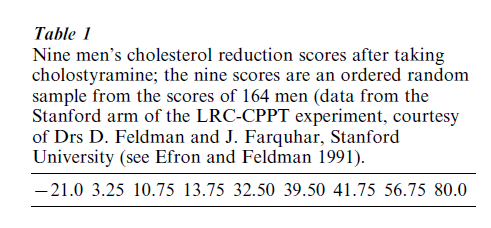
The following fundamental question arises in almost every statistical data analysis: on the basis of a data set z we calculate a statistic s(z) for the purpose of estimating some quantity of interest. For example, z could be the nine cholesterol reduction scores shown in Table 1, and s(z) their mean value z = 28.58, intended as an estimate of the true mean value of the cholesterol reduction scores. (The ‘true mean value’ is the mean we would obtain if we observed a much larger set of scores.) How accurate is s(z)?

This question has a simple answer if s(z) is the mean z of numbers z₁ , z₂ , …, z_n. Then the standard error of z, its root mean square error, is estimated by a formula made famous in elementary statistics courses.

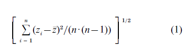
For the nine numbers in Table 1, Eqn. (1) gives 10.13. The estimate of the true cholesterol reduction mean usually would be expressed as 28.58 ±10.13, or perhaps 28.58 ± 10.13•s, where s is some constant like 1.645 or 1.960 relating to areas under a bell-shaped curve. With s = 1.645, interval (2) has approximately 90 percent chance of containing the true mean value.

The bootstrap, (Efron 1979), was introduced primarily as a device for extending Eqn. (1) to estimators other than the mean. For example, suppose s(z) is the ‘25 percent trimmed mean’ z (.25), defined as the average of the middle 50 percent of the data: we order the observations z₁, z₂, …, z_n, discard the lower and upper 25 percent of them, and take the mean of the remaining 50 percent. Interpolation is required for cases where 0.25•n is not an integer. For the cholesterol data, z {.25} = 27.81.

Table 1 Nine men’s cholesterol reduction scores after taking cholostyramine; the nine scores are an ordered random sample from the scores of 164 men (data from the Stanford arm of the LRC-CPPT experiment, courtesy of Drs D. Feldman and J. Farquhar, Stanford University (see Efron and Feldman 1991).

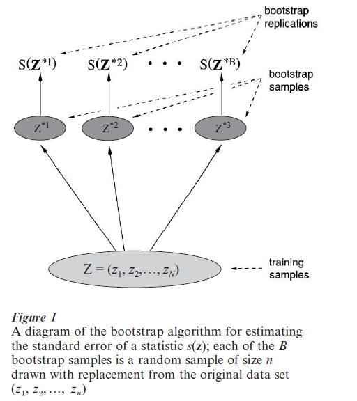
There is no neat algebraic formula like Eqn. (1) for the standard error of a trimmed mean, or for that matter almost any estimate other than the mean. That is why the mean is so popular in statistics courses. In lieu of a formula, the bootstrap uses computational power to get a numerical estimate of the standard error. The bootstrap algorithm depends on the notion of a bootstrap sample, which is a sample of size n drawn with replacement from the original data set z = (z₁, z₂, …, z_n). The bootstrap sample is denoted z* = (z₁, z₂, …, z_n). Each z_i^* is one of the original z values, randomly selected, perhaps z*₁ = z₇, z*₂ = z₅, z*₃ = z₅ , z₄* = z₉, z*₅ = z₇, etc. The name bootstrap refers to the use of the original data set to generate ‘new’ data sets z*.

The bootstrap estimate of standard error for z {0.25} is computed as follows: (a) a large number ‘B’ of independent bootstrap samples each of size n, is generated using a random number device; (b) the 25 percent trimmed mean is calculated for each bootstrap sample; (c) the empirical standard deviation of the B bootstrap trimmed means is the bootstrap estimate of standard error for z {0.25} . Figure 1 shows a schematic diagram of the bootstrap algorithm, applied to a general statistic s(z).

Trying different values of B gave these bootstrap estimates of standard error for the 25 percent trimmed mean applied to the cholesterol data Ideally we would like B to go to infinity. However, it can be shown that randomness in the bootstrap standard error that comes from using a finite value of B is usually negligible for B greater than 100. ‘Negligible’ here means small relative to the randomness caused by variations in the original data set z. Even values of B as small as 25 often give satisfactory results. This can be important if the statistic s(z) is difficult to compute, since the bootstrap algorithm requires about B times as much computation as s(z).

The bootstrap algorithm can be applied to almost any statistical estimation problem. (a) The individual data points z_i need not be single numbers; they can be vectors, matrices, or more general quantities like maps or graphs. (b) The statistic s(z) can be anything at all, as long as we can compute s(z*) for every bootstrap data set z*. (c) The data set ‘z’ does not have to be a simple from a single distribution. Other data structures, for example, regression models, time series, or stratified samples, can be accommodated by appropriate changes in the definition of a bootstrap sample. (d) Measures of statistical accuracy other than the standard error, for instance biases, mean absolute value errors, and confidence intervals, can be calculated at the final stage of the algorithm. These points are discussed in Efron and Tibshirani (1993). The more complicated example below illustrates some of them.

There is one statistic s(z) for which we don’t need the computer to calculate the bootstrap standard error, namely the mean z. In this case it can be proved that as B goes to infinity, the bootstrap standard error estimate goes to √ (n – 1)/n times Eqn. (1). The factor √ (n-1)/n, which equals 0.943 for n = 9, could be removed by redefining the last step of the bootstrap algorithm, but there is no general advantage in doing so. For the statistic z, using the bootstrap algorithm is about the same as using Eqn. (1).

At a deeper level it can be shown that the logic that makes Eqn. (1) a reasonable assessment of standard error for z, applies just as well to the bootstrap as an assessment of standard error for a general statistic s(z). In both cases we are assessing the standard error of the statistic of interest by the ‘true’ standard error that would apply if the unknown probability distribution yielding the data exactly equalled the empirical distribution of the data. The efficacy of this simple estimation principle has been verified by a large amount of theoretical work in the statistics literature of the 1990s (see the discussion and references in Efron and Tibshirani 1993).

Why would we consider using a trimmed mean rather than z itself? The theory of robust statistics, developed since 1960, shows that if the data z comes from a long-tailed probability distribution, then the trimmed mean can be substantially more accurate than z, that is, it can have substantially smaller standard error (see, e.g., Huber 1964). The trouble, of course, is that in practice we don’t know a priori whether or not the true probability distribution is long-tailed. The bootstrap can help answer this question.

Figure 2 shows the bootstrap estimates of standard error for 5 different trimmed means z{p}, ‘p’ being the proportion of the data trimmed off each end of the sample before the mean is taken. (So z {0} is z, the usual mean, while z {0.5} is the median.) These were computed using the bootstrap algorithm in Fig. 1, B = 400, except that at step 2 five different statistics were evaluated for each bootstrap sample z*, namely z{0}, z {0.10}, z {0.25}, z {0.40}, and z {0.50}.

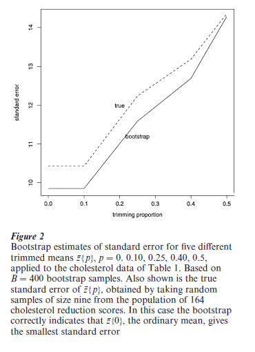
According to the bootstrap standard errors in Fig. 2, the ordinary mean has the smallest standard error among the five trimmed means. This seems to indicate that there is no advantage to trimming for this particular data set.

In fact the nine cholesterol reduction scores in Table 1 were a random sample from a much bigger data set: 164 scores, corresponding to the 164 men in the Stanford arm of a large clinical trial designed to test the efficiency of the cholesterol-reducing drug called cholestyramine (Efron and Feldman 1991). With all of this extra data available, we can check the bootstrap standard errors. The solid line in Fig. 2 indicates the true standard errors for the five trimmed means, ‘true’ meaning the standard error of random samples of size nine taken from the population of 164 scores.

We see that the true standard errors confirm the bootstrap conclusion that the ordinary mean is the estimator of choice in this case. The main point here is that the bootstrap estimates use only the data in Table 1, while the true standard errors require extra data that usually isn’t available in a real data analysis problem.

2. Growth Curves

Longitudinal data are often modeled using growth curves. Our example uses educational testing data from students in North Carolina (see Williamson et al. 1991, Rogosa and Saner 1995). The data we use for the example are eight yearly observations on achievement test scores in mathematics Y for 277 females, each followed from grade 1 to grade 8. The straight-line growth curve model for each individual can be written as

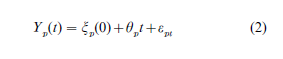
where the observable scores Y contain error of measurement indicated by ε_pt. Here t denotes time and p denotes person. The constant rate of change for each person is indicated by θ_p; θ_p has a distribution over persons with mean µ_θ and variance σ_θ².

To illustrate bootstrap estimation we pick out two of the questions that are investigated using the growth curve models:

(a) Can individual change be measured reliably? In behavioral and social science research the reliability index for the estimated rate of change, ρ(θ), is the parameter of interest.

(b) Is there a relation between initial standing (math achievement in grade 1) and the rate of improvement? The parameter to be estimated is correlation between θ and initial status (over the population of individuals), written as ρ_{θξ( ).}

Maximum-likelihood estimates of ρ(θ) and ρ_{θξ( )} can be obtained from standard mixed model analyses. Standard errors and interval estimates for these quantities are not available from widely-used computer packages.

Figure 3 shows histograms for 4000 bootstrap estimates of ρ(θ) and ρ_{θξ( ).} Bootstrap samples were constructed by resampling individuals (where the data for each individual is a vector of the eight observations). The 90 percent confidence intervals were obtained using the so-called ‘percentile method’: the endpoints are the 0.05 and 0.95 percentiles of the bootstrap histograms. (The percentile method is the simplest of a number of methods for confidence interval construction via the bootstrap: a generally better method is the ‘BC_a’; see Efron and Tibshirani 1993, chap. 12–14. The results in Table 2 show good precision for estimation of the reliability, but relatively less precision for the correlation parameter.

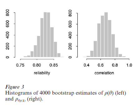
Table 2 Results for growth curve example

3. Related Methods

There are a number of important related methods, with strong similarities to the bootstrap. The jackknife systematically deletes one or more observations from the dataset, and applies the statistic to the remaining data. By doing this for each observation or groups of observations, one can obtain estimates of standard errors and bias that roughly approximate to the bootstrap estimates.

Crossalidation is similar to the jackknife but is used to assess the prediction error of a model. It systematically excludes one or more observations from the dataset, fits the model to the remaining data, and then predicts the data that was left out. Application of the bootstrap for estimating prediction error is not straightforward and requires some special modifications. With these, the bootstrap and cross-validation have similar performance for estimating prediction error. Details and references are given in Efron and Tibshirani (1993) and Efron & Tibshirani (1997).

There is a connection of the bootstrap to Bayesian inference. Roughly speaking, the bootstrap distribution approximates a nonparametric posterior distribution, derived using a noninformative prior. Rubin (1981) gives details.

A difficult theoretical question is: when does the bootstrap work? There is much research on this question (see, e.g., Hall 1992). In ‘regular’ problems where asymptotic normality can be established, first and higher order correctness of the bootstrap (and modifications) have been proven. However, the bootstrap can fail, for example, when it is used to estimate the variance of the maximum or minimum of a sample. More generally, it is difficult to prove theoretically that the bootstrap works in complicated problems: but these are the very settings in which the bootstrap is needed most. Eventually, theory will start to catch up with practice. In the meantime, the bootstrap, like any statistical tool, should be applied with care and in the company of other statistical approaches.

Some popular statistics packages have bootstrap functions, including S-PLUS and Resampling Stats. In most packages that facilitate some customization by the user, it is easy to write one’s own bootstrap function.

4. Conclusions

The bootstrap is a powerful tool for data analysis, with many applications in the social sciences. It is being used more and more, as fast computational tools and convenient software become widely available. Good general references on the bootstrap include Efron and Tibshirani (1993), Davison and Hinkley (1997), Hall (1992), Shao and Tu (1995), and Westfall and Young (1993).

Bibliography:

1. Davison A C, Hinkley D V 1997 Bootstrap Methods and their Application. Cambridge University Press, Cambridge, UK
2. Efron B 1979 Bootstrap methods: Another look at the jack-knife. Annals of Statistics 7: 1–26
3. Efron B, Feldman D 1991 Compliance as an explanatory variable in clinical trials. Journal of the American Statistical Association 86: 9–26
4. Efron B, Tibshirani R 1993 An Introduction to the Bootstrap. Chapman and Hall, London
5. Efron B, Tibshirani R 1997 Improvements on cross-validation: The 632 bootstrap method. Journal of the American Statistical Association 92: 548–60
6. Hall P 1992 The Bootstrap and Edgeworth Expansion. SpringerVerlag, Berlin
7. Huber P 1964 Robust estimation of a location parameter. Annals of Mathematics and Statistics 53: 73–101
8. Rogosa D R, Saner H M 1995 Longitudinal data analysis examples with random coefficient models. Journal of Educational and Behavioral Statistics 20: 149–70
9. Rubin D 1981 The Bayesian bootstrap. Annals of Statistics: 130–134
10. Shao J, Tu D 1995 The Jack-knife and Bootstrap. SpringerVerlag,
11. Westfall P H, Young S S 1993 Resampling-based Multiple Testing: Examples and Methods for palue Adjustment. Wiley
12. Williamson G, Appelbaum M, Epanchin A 1991 Longitudinal analyses of academic achievement. Journal of Educational Measurement 1: 61–76