Discrete Multivariate Analysis Research Paper

1. Traditional Analyses Of Discrete Multivariate Data

Most commonly, discrete variables are categorical in nature. That is, the measurement scale is a set of categories, such as (liberal, moderate, conservative) for political philosophy. In multivariate analyses with two or more categorical variables, a contingency table displays the counts for the cross-classification of categories. For instance, a contingency table might display counts indicating the number of subjects classified in each of the 9 = 3 × 3 combinations of responses on political philosophy and political party orientation (Democrat, Republican, Independent). Those combinations form the cells of the table.

Two categorical variables are independent if the probability of response in any particular category of one variable is identical for each category of the other variable. This is an idealized situation that is rarely true in practice, although like any statistical model it is sometimes adequate for describing reality. For instance, some surveys of American college students have shown that opinion about whether abortion should be legal is essentially independent of gender; that is, the percentage favoring legalization is about the same for male and female students.

Treating independence as a simple model for a contingency table, we can test its fit using statistics that compare the observed cell counts in the table to those expected (predicted) by that model. The most commonly used test statistics are

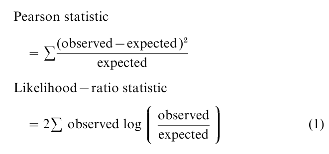
These both have large-sample chi-squared distributions. For r rows and c columns, the degrees of freedom (df) for the test equal df = (r – 1)(c – 1), and the P-value is the right-tail probability above the observed test statistic value. These chi-squared statistics also can compare counts to expected values for more complex models than independence.

In conducting goodness-of-fit tests, one does not seriously entertain the possibility that the model truly holds; any model is false and provides a simple representation that only approximates reality. However, when the chi-squared statistics do not show significant lack of fit, benefits of model parsimony accrue from using the model fit, which smooths the sample cell proportions somewhat. Interpretations are simpler, and estimates of population characteristics such as the true cell proportions are likely to be better using the model-based estimates.

Multidimensional contingency tables result from cross-classifying more than two categorical variables, such as for studying the association separately at levels of control variables race, gender, or educational level. The model of conditional independence states that two categorical variables are independent at each level of a third; that is, ordinary independence applies in each partial table. Large-sample chi-squared tests of fit of this model, such as the Cochran–Mantel–Haenszel test, combine the information from the partial tables. Most are designed to be relatively powerful when the strength of the association is similar in each partial table. The model of homogeneous association states that the strength of association between two variables is identical at each level of a third variable. Goodnessof-fit tests of these models were originally formulated for stratified two-by-two tables, but generalizations exist for stratified r-by-c tables with ordered or unordered categories

Goodness-of-fit tests have limited use, and in many circumstances it is more informative to estimate the strength of the associations. Goodman and Kruskal (1979) discussed a variety of summary measures. Those for ordinal variables, such as their gamma measure, are correlation-like indices that fall between – 1 and + 1. More attention has been focused on measures that arise as parameters in models. The odds ratio, discussed in the next section, is a parameter in logistic regression and loglinear models and is applicable for two-way or multi-way tables.

For estimating parameters in models for discrete data, the method of maximum likelihood estimation is the standard. The probability function for the data (e.g., Poisson, binomial), expressed as a function of the parameters after observing the data, is called the likelihood function. The maximum likelihood estimates are values for the parameters for which this achieves its maximum; that is, these estimates are the parameter values for which the probability of the observed data takes its maximum value. Except in a few simple cases, numerical methods are needed to find the maximum likelihood estimates and their standard errors. Soft- ware is reasonably well developed in the major statistical packages. It is often most natural to analyze discrete data using procedures for generalized linear models that permit non-normal responses, such as the Poisson and binomial. Examples include PROC GENMOD in SAS and the ‘glm’ function in S-Plus. For instance, for SAS see Allison (1999) and Stokes et al. (1995), for S-Plus see Venables and Ripley (1999), and for Stata see Rabe-Hesketh and Everitt (2000).

2. Regression Modeling Of A Categorical Response

For multidimensional contingency tables and other forms of multivariate data, modeling approaches are vital for investigating association and interaction structure. Logistic regression is an analog of ordinary regression for binary response variables, and it has extensions for multicategory response variables. Like ordinary regression, logistic regression distinguishes between response and predictor variables. The predictor variables can be qualitative or quantitative, with qualitative ones handled by dummy variables.

Let p denote the probability of outcome in a particular response category (e.g., favoring the Democratic rather than Republican candidate for President). For the observations at particular fixed values of predictor variables, the number of responses in the two outcome categories is assumed to have the binomial distribution. With a set of predictors x₁, x₂,…, x_p, the logistic regression model is

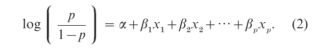
The ratio p/(1 – p) is called the odds, and the natural logarithm of the odds is called the logit.

One reason for using the logit instead of p itself on the left-hand side of this equation is to constrain predicted probabilities to fall between 0 and 1. With a single predictor, for instance, the linear probability model p = α + βx permits p to fall below 0 or above 1 for many values of x; by contrast, the formula log[ p/(1 – p)] = α + βx maps out an S-shaped function for which p increases or decreases according to whether β > 0 or β < 0 but always stays bounded between 0 and 1. For instance, for the decision to buy rent a home, suppose the relationship between p = the probability of buying and x annual family income (in ten thousands of dollars) satisfies the logistic regression model log[p/(1 – p)] = 4.0 – 0.8x. Figure 1 shows the plot of p for x between 0 and 10 (i.e., below $100,000). The plot is roughly linear for p between 0.2 and 0.8.

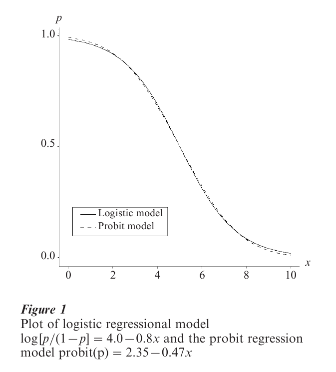
The probit model is another model that has this S- shape. The function probit ( p) = α + βx has a graph for p (or for 1 – p when β < 0) that has the shape of a normal cumulative distribution function with mean -α/β and standard deviation 1/|β|. The probit model can be derived by assuming an underlying latent normal variable (e.g., Long 1997). In practice, the probit model gives a very similar fit to the logistic regression model. To illustrate, Fig. 1 also shows the plot of the equation probit ( p) = 2.35 – 0.47x, which has the shape of a normal cumulative distribution function with mean 5.0 and standard deviation 2.1; for instance, a decrease in p of 0.68, from p = 0.84 to p = 0.16, occurs between x = 5.0 – 2.1 = 2.9 and x = 5.0 + 2.1 = 7.1. Although the fits are very similar, estimates of α and β are on a different scale for probit and logistic models, and usually logistic parameter estimates are about 1.6 to 1.8 times the probit parameter estimates.

With multiple predictors, the coefficient β_k of x_k in the logistic regression model describes the effect of x_k, controlling for the other predictors in the model. The antilog of β_k is an odds ratio representing the multiplicative effect of a one-unit change in x_k on the odds. For instance, in a model for the probability in favoring the Democratic candidate for President, suppose β_k = 0.40 for the coefficient of x_k = gender, with x_k = 1 for females and 0 for males. Then, controlling for the other variables in the model, for females the odds of favoring the Democratic candidate equal e^0.40 = 1.49 times the odds for males; that is, the odds of favoring the Democrat are 49 percent higher for females than for males.

For quantitative predictors, simple interpretations that apply directly to the probability p rather than to the odds p/(1 – p) result from straight-line approximations to the logistic S-shaped curve for p. When p is near 0.5, β_k/4 is the approximate change in p for a one-unit change in x_k, controlling for the other predictors. To illustrate, suppose β_k = – 0.12 for the coefficient of x_k = annual income (in ten thousands of dollars) in the model for the probability of favoring the Democratic candidate. Then, for an increase of $10,000 in income near where p = 0.5, the probability of support for the Democratic candidate decreases by about 0.12/4 = 0.03, other variables being kept constant. To test the effect of a term in the model, the ratio of the estimate of β_k to its standard error has an approximate standard normal distribution, under the hypothesis of no effect (H₀: β_k = 0).

Using the estimated parameters from the logistic regression model, one can also estimate the probability p for given settings for the predictors, as

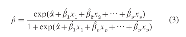
When all predictors are categorical, chi-squared tests analyse the adequacy of the model fit by comparing the observed cell counts to values expected under the model.

Generalizations of logistic regression apply to categorical response variables having more than two categories. A multicategory extension of the binomial distribution, called the multinomial, applies to the response counts at each setting of the predictors.

For nominal responses, the generalized model forms logits by pairing each response category with a baseline category. For a r-category response, the model has form

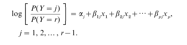
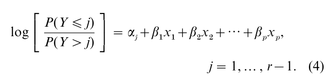
A separate set of parameters applies for each response category contrasted with the final one. For instance, if Y refers to preferred candidate and has categories (Democrat, Republican, Independent), the effect of gender on the choice between Democrat and Independent may differ from its effect on the choice between Republican and Independent. The choice of category for the baseline (the denominator of the logits) is arbitrary. Regardless of this choice the same inference occurs about comparisons of models with and without certain predictors and about estimated probabilities in the r response categories. For ordinal responses, the cumulatie logit model describes the effects of predictors on the odds of response below any given level instead of above it (i.e., the model refers to an odds for the cumulative probability; see McCullagh 1980). It has form

For further details about logistic regression models, see Multivariate Analysis: Discrete Variables (Logistic Regression); also Agresti (1996, Chap. 5), Collett (1991) Hosmer and Lemeshow (2000) and Long (1997).

3. Loglinear Models

Logistic regression resembles ordinary regression in distinguishing between a response variable Y and a set of predictors {x_k}. Loglinear models, by contrast, treat all variables symmetrically and are relevant for analyses analogous to correlation analyses, studying the association structure among a set of categorical response variables.

For multidimensional contingency tables, a variety of models are available, varying in terms of the complexity of the association structure. For three variables, models include ones for which (a) the variables are mutually independent, (b) two of the variables are associated but are jointly independent of the third, (c) two of the variables are conditionally independent, given the third variable, but may both be associated with the third, (d) each pair of variables is associated, but the association between each pair is homogeneous at each level of the third variable, and (e) each pair of variables is associated and the strength of association between each pair may vary according to the level of the third variable (Bishop et al. 1975).

Relationships describing probabilities in contingency tables are naturally multiplicative, so ordinary regression-type models occur after taking the logarithm, which is the reason for the term loglinear. To illustrate, in two-way contingency tables independence between row variable X and column variable Y is equivalent to the condition whereby the probability of classification P(X = i, Y =j ) in the cell in row i and in column j depends only on the marginal probabilities P(X = i ) and P(Y = j ),

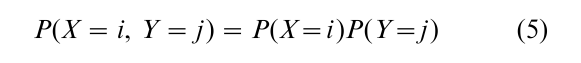
for all i and j. For a sample of size n, the expected count µ_ij = nP(X = i, Y =j ) in that cell therefore satisfies

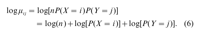
This has the loglinear form

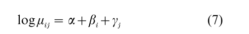
for which the right-hand side resembles a simple linear model—two-way analysis of variance (ANOVA) with- out interaction. Alternatively this has regression form by replacing {β_i} by dummy variables for the rows

 times parameters representing effects of classification in those rows and replacing {γ_j} by dummy variables for the columns times parameters representing effects of classification in those columns.

Similarly, loglinear model formulas for more complex models such as those allowing associations resemble ANOVA models except for predicting the logarithm of each cell expected frequency rather than the expected frequency itself. Dummy variables represent levels of the qualitative responses, and their interaction terms represent associations. The associations are described by odds ratios. Logistic regression models with qualitative predictors are equivalent to certain loglinear models, having identical estimates of odds ratios and identical goodness-of-fit statistics. For ordinal variables, specialized loglinear models assign ordered scores to the categories and have parameters describing trends in associations.

For further details about loglinear models, see Exploratory Data Analysis: Multivariate Approaches (Nonparametric Regression); also Agresti (1996, Chap. 6), Bishop et al. (1975), and Fienberg (1980).

4. Sampling Assumptions

Inferential analysis of multivariate discrete data, like that of any type of data, requires assumptions about the sampling mechanism that generated the data. Often, such as in most surveys, the overall sample size is fixed and the multinomial distribution applies as the probability distribution for the counts in a contingency table. In many cases, certain marginal totals are also fixed, such as in experimental designs in which the number of subjects at each experimental condition is fixed. In addition, in regression-type models such as logistic regression, it is common to treat the counts at the combinations of levels of the predictor variables as fixed even if they are not fixed in the sampling design. In these cases, at each such combination the response is usually assumed to have a binomial distribution when the response is binary and a multinomial distribution when the response is multicategory; this replaces the usual normal response assumption for regression models for continuous responses. Other sampling possibilities, less common in practice, are that the sample size is itself random (i.e., no counts are fixed, such as in observing categorical outcome measures for all subjects who visit some clinic over a future time period) or, at the other extreme, all marginal totals are fixed; these lead to Poisson and hypergeometric distributions.

Although some methods depend on the sampling assumption, estimates and test statistics for many analyses are identical for the common sampling designs. For instance, for two-way contingency tables, the chi-squared statistic, its degrees of freedom, and its large-sample P-value are the same when only the total sample size is fixed, when only the row totals are fixed, when only the column totals are fixed, or when both row and column totals are fixed.

Under standard sampling assumptions, traditional methods of inference for discrete data use statistics having approximate chi-squared or normal distributions for large samples. Alternative methods are available for small samples. Fisher’s exact test, due to the famous statistician R. A. Fisher, is a test of independence in 2-by-2 contingency tables. Analogs of this test are available for larger tables and for testing conditional independence and homogeneous association in three-way tables (characterized in terms of homogeneity of odds ratios) as well as testing fit of more complex logit and loglinear models. Small sample confidence intervals for parameters such as proportions, difference of proportions, and odds ratios, result from inverting exact tests for various null values of parameters. Much of the current research in small-sample inference uses simulation methods to closely approximate the true sampling distributions of relevant statistics (e.g., Forster et al. 1996). StatXact (Cytel Software 1999) is statistical software dedicated to small-sample discrete-data methods. Some of these analyses are also available in modules of software such as SAS and SPSS.

5. Alternative Model Types

For contingency tables relating several response variables, alternative statistical approaches to loglinear models can describe association among the variables. Foremost among these is correspondence analysis, a graphical way of representing associations in two-way contingency tables that has been particularly popular in France (e.g., Benzecri 1973; see Multivariate Analysis: Discrete Variables (Correspondence Models). The rows and columns are represented by points on a graph, the positions of which indicate associations between the two. Goodman (1986) developed a modelbased version of this approach. He showed it has equivalences with correlation models, which determine scores for categories that maximize correlations between categorical variables. He also showed approximate connections with a set of association models that he helped to develop, some of which have loglinear model form but with scores or score-like parameters assigned to levels of ordinal variables. Clogg and Shihadeh (1994) surveyed such models.

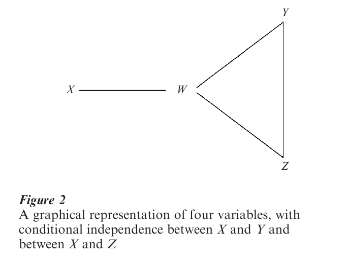
Another graphical way of representing a multivariate relationship uses graphical models that study conditional independence structure among the variables. Roughly speaking, the graph has a set of vertices, each vertex representing a variable. An edge connecting two vertices represents a conditional association between the corresponding two variables. For instance, for four variables, the graph in Fig. 2 portrays a model that assumes that X and Y are independent and that X and Z are independent, conditional on the remaining two variables, but permits association between W and X and between each pair of variables in the set {W, Y, Z}. The four edges in the graph, connecting W and X, W and Y, W and Z, and Y and Z, represent pairwise conditional associations. Edges do not connect X and Y or X and Z, since those pairs are conditionally independent. Many loglinear models are graphical models. For details, see Lauritzen (1996) and Graphical Models: Overview.

Logistic/probit regression models and loglinear models, together with long-established regression and ANOVA methods for normal response variables, are special cases of a broad family of generalized linear models (Gill 2000). These models are characterized by a choice of distribution for the response variable (e.g. binomial, Poisson, normal), a function of the mean to be modeled (e.g., logit of the mean, log of the mean, the mean itself ), and the variables that enter the linear model formula as predictors.

For binary data, the model using the logit transform of the probability p is the most popular generalized linear model. For count data, generalized linear models usually assume a Poisson response, sometimes called Poisson regression models. However, more variability often occurs in the counts than the Poisson distribution allows (i.e. there is said to be overdispersion). The Poisson distribution forces the variance to equal the mean; according to it, for instance, at a given mean for Y the variance of the conditional distribution of Y cannot change as predictors are added to or deleted from the model. Methods of dealing with overdispersion include using discrete distributions for which the variance can exceed the mean, such as the negative binomial, and adding an extra error term to the model (a random effect) to account for unexplained variability due to factors such as unmeasured variables and measurement error.

Extensions of generalized linear models deal with more complex situations. For instance, sometimes the response is a mixture of discrete and continuous, such as when a certain proportion of the responses take value 0 but the rest can be any positive real number (e.g., responses to ‘How much time do you spend on exercise each week?’). Sometimes observations are censored—we know only that the response falls above some point or below some point, such as when we count events of a certain type over time but cannot observe beyond the end of the experimental period (Andersen et al. 1993). Models can then focus on the continuous time to response of an event or the discrete counting of events. Depending on the application and the sort of censoring, the models have different names, including survival models, event-history models, and tobit models (e.g., Long 1997).

6. New Methods For Repeated Measurement Data

For standard inference with the usual sampling assumptions, the methods discussed above treat separate observations in a sample as independent. In the social and behavioral sciences, multivariate data often results from repeated measurement (e.g., longitudinal) studies. For such studies, this independence assumption is violated. More generally, data sets that consist of clusters of observations such that observations within clusters tend to be more alike than observations between clusters require specialized methods. This was an active research area in the last 15 years of the twentieth century. New methods make it possible to extend traditional repeated measures ANOVA to discrete data and to permit various correlation structures among the responses.

For clustered data, recently developed methods enable modeling binary or categorical responses with explanatory variables, for instance using the logit transform. Two approaches have received considerable attention. In one, models address marginal (separate) components of the clustered response, allowing for dependence among the observations within clusters but treating the form of that dependence as a nuisance that is not a primary object of the modeling. The other approach uses cluster-specific random effects as a mechanism for inducing the dependence.

The marginal modeling approach has the advantage of relative computational simplicity. Estimates are obtained using the methodology of generalized estimating equations (see Diggle et al. 1994). With this quasi-likelihood method, rather than fully specify joint distributions for the responses, one need only model how the variance depends on the mean and predict a within-cluster correlation structure. A simple version of the method exploits the fact that good estimates of regression parameters usually result even if one naively treats the component responses in a cluster as independent. Although those parameter estimates are normally adequate under the naıve independence assumption, standard errors are not. More appropriate standard errors result from an adjustment using the empirical dependence in the sample data. Although one makes a ‘working guess’ about the likely correlation structure, one adjusts the standard errors to reflect what actually occurs for the sample data. An exchangeable working correlation structure under which correlations for all pairs of responses in a cluster are identical is more flexible and usually more realistic than the naıve independence assumption.

With models that apply directly to the marginal distributions, the regression effects are population-averaged. For instance, a fitted probability estimate refers to all subjects at the given level of predictors, and the model does not attempt to study potential heterogeneity among the subjects in this probability. Alternatively, one can model subject-specific probabilities and allow such heterogeneity by incorporating subject or cluster random effects in the model. For instance, a model might contain a cluster-specific intercept term that varies among clusters according to some normal distribution. The estimated variance of that distribution describes the extent of heterogeneity. This type of model is called a generalized linear mixed model since it contains a mixture of fixed and random effects. Specifying this form of model also has implications about the effects in a marginal model, but the form of model may differ. For instance, with random effects in a logistic regression model, the corresponding model for marginal distributions is only approximated by a logit model and the effects have different size (Diggle et al. 1994).

An alternative approach of dealing with the cluster terms is the fixed effects one of item response models such as the Rasch model. In some applications with a multivariate response, it is natural to assume the existence of an unmeasured latent variable that explains the association structure. Conditional on the value of that latent variable, the observed variables are independent. The observed association structure then reflects association between the observed variables and that latent variable. When the latent variable consists of a few discrete classes, such as when the population is a mixture of a few types of subjects, then the resulting model is called a latent class model. This is an analog of factor analysis in which the observed and latent variables are categorical rather than continuous. See Heinen (1993) and Factor Analysis and Latent Structure: Overview.

7. Historical Notes

The early development of methods for discrete multivariate data took place in England. In 1900, Karl Pearson introduced his chi-squared statistic (although in 1922 R. A. Fisher showed that Pearson’s df formula was incorrect for testing independence) and G. Udny Yule presented the odds ratio and related measures of association. Much of the early literature consisted of debates about appropriate measures of association for contingency tables. Goodman and Kruskal (1979) surveyed this literature and made significant contributions of their own.

In the 1950s and early 1960s, methods for multidimensional contingency tables received considerable attention. These articles were the genesis of substantial research on logistic regression and loglinear models between about 1965 and 1975. Much of the leading work in that decade took place at the universities of Chicago, Harvard, and North Carolina. At Chicago, Leo Goodman wrote a series of groundbreaking articles for statistics and sociology journals that popularized the methods for social science applications. Simultaneously, related research at Harvard by students of Frederick Mosteller (such as Stephen Fienberg) and William Cochran and at North Carolina by Gary Koch and several students and coworkers was highly influential in the biomedical sciences.

Perhaps the most far-reaching contribution was the introduction by British statisticians John Nelder and R. W. M. Wedderburn in 1972 of the concept of generalized linear models. This unifies the primary categorical modeling procedures—logistic regression models and loglinear models—with long-established regression and ANOVA methods for normal-response data.

Texts covering logistic regression are, from least to most advanced, Agresti and Finlay (1997, Chap. 15), Agresti (1996), Hosmer and Lemeshow (2000), Collett (1991), Long (1997), Agresti (1990). Texts covering loglinear models, from least to most advanced, are Agresti and Finlay (1997, Chap. 15), Agresti (1996), Fienberg (1980), Clogg and Shihadeh (1994), Agresti (1990), Bishop et al. (1975). Andersen (1980) and Long (1997) discuss some alternative methods for discrete data.

Bibliography:

1. Agresti A 1990 Categorical Data Analysis. Wiley, New York
2. Agresti A 1996 An Introduction to Categorical Data Analysis. Wiley, New York
3. Agresti A, Finlay B 1997 Statistical Methods for the Social Sciences, 3rd edn. Prentice-Hall, Upper Saddle River, NJ
4. Allison P D 1999 Logistic Regression Using the SAS System. SAS Institute, Cary, NC
5. Andersen E B 1980 Discrete Statistical Models with Social Science Applications. North Holland, Amsterdam
6. Andersen P K, Borgan Ø, Gill R D, Keiding, N 1993 Statistical Models Based on Counting Processes. Springer, New York
7. Benzecri J-P 1973 L’analyse des Donnees. Dunod, Paris
8. Bishop Y M M, Fienberg S E, Holland P W 1975 Discrete Multivariate Analysis. MIT Press, Cambridge, MA
9. Clogg C C, Shihadeh E S 1994 Statistical Models for Ordinal Variables. Sage, Thousand Oaks, CA
10. Collett D 1991 Modelling Binary Data. Chapman and Hall, London
11. Cytel Software 1999 StatXact, Version 4. Cambridge, MA
12. Diggle P J, Liang K-Y, Zeger S L 1994 Analysis of Longitudinal Data. Oxford University Press, Oxford
13. Fienberg S E 1980 The Analysis of Cross-classified Categorical Data, 2nd edn MIT Press, Cambridge, MA
14. Forster J J, McDonald, J W, Smith, P W F 1996 Monte Carlo exact conditional tests for log-linear and logistic models. Journal of the Royal Statistical Society, Series B 58: 445–53
15. Gill J 2000 Generalized Linear Models: A Unified Approach. Sage, Thousand Oaks, CA
16. Goodman L A 1986 Some useful extensions of the usual correspondence analysis approach and the usual log-linear models approach in the analysis of contingency tables. International Statistical Review 54: 243–70
17. Goodman L A, Kruskal W H 1979 Measures of Association for Cross Classifications. Springer, New York
18. Heinen T 1993 Discrete Latent Variable Models. Tilburg University Press, The Netherlands
19. Hosmer D W, Lemeshow S 2000 Applied Logistic Regression, 2nd edn., Wiley, New York
20. Lauritzen, S L 1996 Graphical Models. Oxford University Press, Oxford
21. Long J S 1997 Regression Model for Categorical and Limited Dependent Variables. Sage, Thousand Oaks, CA
22. McCullagh P 1980 Regression models for ordinal data. Journal of the Royal Statistical Society, Series B 42: 109–42
23. Rabe-Hesketh S, Everitt B 2000 A Handbook of Statistical Analyses Using Stata, 2nd edn. CRC Press, London
24. Stokes M E, Davis C E, Koch G G 1995 Categorical Data Analysis Using the SAS System. SAS, Cary, NC
25. Venables W N, Ripley B D 1999 Modern Applied Statistics with S-Plus, 3rd edn. Springer, New York