Multilevel Methods of Statistical Analysis Research Paper

Several generalized regression methods are commonly used in the analysis of hierarchical data. Hierarchical or random coefficient models are multilevel. So too are fixed effects models, marginal models, classical single-level estimation followed by regression coefficient covariance matrix adjustment, and hybrid approaches. The choice of an approach for a particular research problem must depend on the goals of the research and assessment of the design and measurement deficiencies presented by a particular body of data, and is often consequential. Multilevel modeling approaches emphasize different aspects of the data, vary in the nature and stringency of their assumptions, and support different kinds of descriptions and interpretations. Poor choice of method can lead to the application of an incorrectly specified model, and thereby to good estimates of the wrong quantities.

1. Random Coefficient Models

The random coefficient model offers a compelling formulation that is consistent with the social scientific goal of understanding how units at one level affect, and are affected by, units at other levels. Consider a design with two levels, and suppose that there is a single level-1 regressor (X ), a single level-2 regressor (G) that is by definition constant over all level-1 observations within a context, and that the dependent variable (Y ) is Gaussian distributed conditional on X and G. The random coefficient model can be expressed as

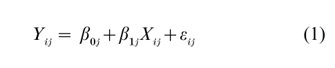
with

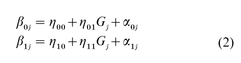
where j= 1, 2,…, J denotes contexts (level-2 units), and i = 1, 2,…, n_j denotes individuals within contexts (level-1 units). The level-2 equations (Eqn. (2)) assert that the level-1 intercepts and slopes vary over contexts as linear functions of G. There is often justification for supposing that the within-context coefficients depend on contextual characteristics. It is appealing that the dependence includes random error components (α_0j and α_1j).

Assumptions about the error structure of this two- level model are that, for each context, the level-1 errors follow the Gaussian distribution, are centered on zero, have constant variance, and are independent. The error variances may vary over contexts. The level-2 errors are also Gaussian distributed, centered on zero, independent within equations, and have constant variances. The level-2 errors may be correlated across equations. It is further assumed that the level-1 errors are orthogonal to the level-2 errors, and that all error terms are orthogonal to X and G. The orthogonality assumptions are needed to secure consistent estimates of the η’s.

Many generalizations of this model are possible— coefficients can be constrained to be nonrandom; the dependent variable may be discrete, counted, truncated, ordinal, or time to event; there may be more regressors at any level as well as more than two levels; the nesting of levels may be cross-classified; different assumptions about the functional forms of the distributions of the errors can be made; and the assumption of independence of errors within level-2 (or higher) units can be relaxed. Nevertheless, the assumptions of orthogonality between regressors and errors, and of cross-level orthogonality between error components, continue to remain important. Until that is no longer so, the credibility of an application of a random coefficient model rests on the plausibility of these assumptions, which should be thought of as inextricably linked to the systematic components of the model, and not as the fine print of a contract that is never read, much less enforced.

However compelling it may be on substantive grounds to specify the random coefficient multilevel model as Eqns. (1) and (2), substitution of Eqn. (2) into Eqn. (1) results in the equivalent mixed-model representation

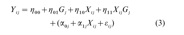
which demonstrates that treating intercepts and slopes as dependent on G is the same as supposing that Y depends on X, G, and their cross-level (product) interaction.

Random coefficient models with Gaussian errors are commonly estimated by maximum likelihood or restricted maximum likelihood. For binary response the prevalent methods are marginal and penalized quasi-likelihood, although Bayesian methods based on Markov Chain Monte Carlo (MCMC) estimation are also beginning to be used. A consensus on preferred methods of estimation of multilevel binary response and other nonlinear (non-Gaussian) models has yet to emerge. Estimation of multilevel models is iterative and computationally intensive, more so for non-Gaussian cases. Especially for these cases, researchers are well advised to check numerical estimates across algorithms, methods, and software. Other problems, such as substantial design imbalance in combination with context size, also need to be evaluated for their potential impact on numerical estimates.

2. Fixed Effects Models

The fixed effects model does not require the assumption of orthogonality between X and α inherent to the random coefficient model. It can be written as

where the δ_j are between-context contrasts, and the u_ij are assumed to be classical Gaussian errors. Relative to the random coefficient model, the additive term in G has been dropped, and the intercept and slope are no longer allowed to vary randomly over contexts, although each context is allowed its own intercept and the cross-level interaction is retained. The δ_j absorb the additive component of all possible G-variables, not just the finite number that can be included in Eqn. (3). Additive components for any level-1 regressors that do not vary within contexts are also absorbed by the δ_j.

In the fixed effects approach, ‘fixing’ the between- context contrasts means that the contexts are them- selves assumed to be fixed, in the sense that statistical inference is conditional on the particular selection of

 contexts present in the data. Because the contrasts can be defined as the coefficients of a set of indicator variables that assign individuals to contexts, there is no need to assume that context membership is orthogonal to X. This is a critical difference between the fixed effect and random coefficient models. If the assumption of orthogonality between X and α is implausible in the random coefficient model, and it can be when the list of G-variables is incomplete, then the fixed effects model provides an alternative that solves the problem. In the Gaussian case, the fixed effects model is a conventional regression model. When J is large—and often when it is not—there may be little interest in describing estimated values of the δ_j, in which case estimation of the other covariate coefficients can be performed after within-context centering of the variables. For a binary response variable, conditional logistic regression can be used to estimate fixed effect models (Chamberlain 1980). In this case, the context contrasts are not estimated, although additive context differences are controlled. Software for fixed effects estimation is widely available.

If it is desired to obtain estimates of the additive component of the contextual variables, then the fixed effects approach is not the method of choice. Also, in the binary response case, conditional logistic regression does not necessarily use all of the data, and in this sense may be inefficient.

3. Coefficient Variance Estimates Adjusted For Clustering

The adjusted coefficient variance estimator in common use for multilevel analysis is a robust estimator. In actual applications, care must be taken to ensure that the robust estimator selected includes an extension of the algorithm for the general robust estimator that accommodates clustering. With the robust estimator, it is possible to specify a model whose systematic component is identical to that of Eqn. (3), and whose error component need not be independently and identically distributed, Gaussian distributed, or orthogonal to the regressors. The robust equivalent of Eqn. (3) can be expressed as:

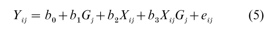
Least-squares computation can be used to produce coefficients whose estimated variances and covariances are subsequently adjusted for context membership. The coefficients will be unbiased estimates of the corresponding terms in Eqn. (3) if the orthogonality assumption is satisfied. The standard errors will be adjusted for clustering and other sources of hetero-scedasticity regardless of whether this is so. When Eqn. (3) is true, confidence intervals for its coefficients obtained by prevailing methods will tend to be smaller than confidence intervals based on the robust clustering adjustment associated with Eqn. (5).

The robust approach is also an alternative to the fixed effects approach. The latter achieves orthogonality between the regressors and the error component by including context membership in the systematic component of the model, but is unable to include main effects of contextual variables even though it controls for all possible contextual variables. In the robust approach coefficients of contextual regressors are estimated, but all possible contextual variables are not controlled. Coefficient standard errors are adjusted for clustering, but the coefficient estimates are not efficient.

The robust, variance adjustment approach to multi- level analysis has been extended to models of discrete and counted outcomes, and to survival problems, and can be used where a fixed effects approach is not available. Nevertheless, where it can be justified, explicit incorporation of clustering into model specification is preferable to post hoc adjustments of estimators that ignore clustering.

4. Marginal Models

When Y is a discrete or count response variable, it is possible to specify a multilevel model in which the within-context correlatedness of observations is in- corporated as a side condition on the model, rather than as a consequence of a random intercept. For Y binary and ω_ij, the logit of ‘success’ for the ijth observation, the multilevel dependence of Y on regressors, can be written as

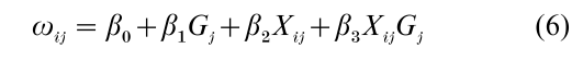
with an additional specification indicating the pattern of correlation between observations within a context (corr(Y_ij, Y_i´j), i = i´). Specifying that all pairs of observations within a context are equally correlated corresponds to the assumption of correlatedness induced by a random coefficient model, but virtually any pattern can be specified.

Models that characterize the marginal distribution of Y as a function of regressors are said to be marginal models. The model of Eqn. (6) and its side condition on correlated observations is a member of this class. The generalized linear model (McCullagh and Nelder 1989), a unifying theoretical framework for the linear model and discrete and count response variables, has been extended to allow for the analysis of multilevel data (Liang and Zeger 1986, Zeger and Liang 1986). This extension, known as the generalized estimating equations approach (GEE), provides a marginal model (population-average) alternative to random coefficient models when Y is discrete or a count. Equation (6) can be estimated using the GEE method.

Gaussian random effects models sustain a marginal model interpretation of regression coefficients. Random effects models for discrete and count response variables do not. Marginal models are appropriate when the analytic goal is to infer how Y depends on covariates for a population of level-1 units averaged over contexts. Random effects models are appropriate when within-context estimates are desired. For the logistic response case, the estimated coefficients of marginal models tend to be smaller in absolute value than the corresponding coefficients in random effects models (Diggle et al. 1994, p. 141).

Marginal models for Y discrete or a count can be estimated for a broad range of structures of potential within-context correlation; random coefficient models for discrete and count response variables currently cannot. Computation is fast (iterative generalized least squares), and estimation is relatively straightforward compared to binary response random coefficient models, although issues surrounding optimal characterization of within-context correlation and estimation of coefficient standard errors continue to attract attention.

5. Omitted Variables

Omitted variables in random coefficient models are of particular concern when they are endogenous, that is, correlated with Y and the included regressors, because they induce coefficient bias. The fixed effect approach provides one solution to this problem when the omitted variables are contextual. There are others: measurement of omitted variables, random assignment to contexts, and instrumental variables estimation.

Measuring the omitted variables is not an option in secondary analysis or in the midst of primary analysis—by then the data have been collected and returning to the field is generally infeasible. This should not, however, preclude future attempts to extend the range of measurement.

Random assignment to contexts presumes that an experimental design is feasible in the study of a particular phenomenon. Often it is not. Even when randomization is possible, it is not necessarily well suited to answering certain kinds of questions.

Instrumental variables estimation is often used in an effort to solve an endogeneity problem. When an instrumental variables approach is used, aspects of the clustering problem may be sacrificed to solve what is perceived as a much more important one—selection into contexts. In Eqn. (3) replace X by T, suppose that the underlying data structure is quasi-experimental, and let T_ij = 1 if an individual is treated (0 otherwise). If Y is a health outcome and contexts are hospitals, and if assignment to treatment is not random, then ε potentially contains unmeasured variables correlated with T and also with Y. In quasi- and nonexperimental data, whether a patient receives a particular kind of treatment can be nonrandom with some causes known, others not. An instrumental variables approach to this problem attempts to find one or more covariates W correlated with T and Y, where Y and W controlling T are uncorrelated, and W and ε are uncorrelated. It is often difficult to find plausible instruments (W ), although contextual variables are sometimes used. Thus, instrumental variables estimation cannot be employed with the automaticity of any of the other approaches to clustered data.

6. Examples

An example of a Gaussian application, and another of a binary response application, illustrate the kinds of differences in findings that can occur using alternative multilevel approaches. The data are from a one percent clustered sample of the 1990 Census of China, and are specific to Hainan province. Clustering is at the enumeration district level, and within clusters enumeration is 100 percent.

6.1 Gaussian Example

In the Gaussian example, there are 17,662 men in the data, distributed over 332 clusters, the smallest having 114 men and the largest having 3,735. The occupational socioeconomic status (SEI) of men ages 20–65 is a function of age and years of schooling at the individual level, type of place of residence (rural vs. urban), and the square of a contextualized measure of education. Type of place of residence is a characterization of place, and constant within contexts. Substantive theory and exploratory data analysis lead to this random effects model:

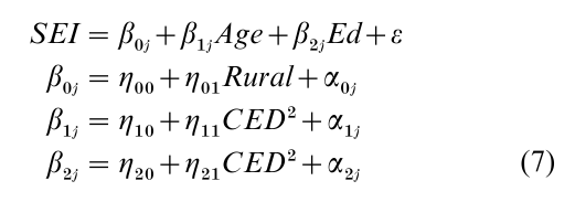
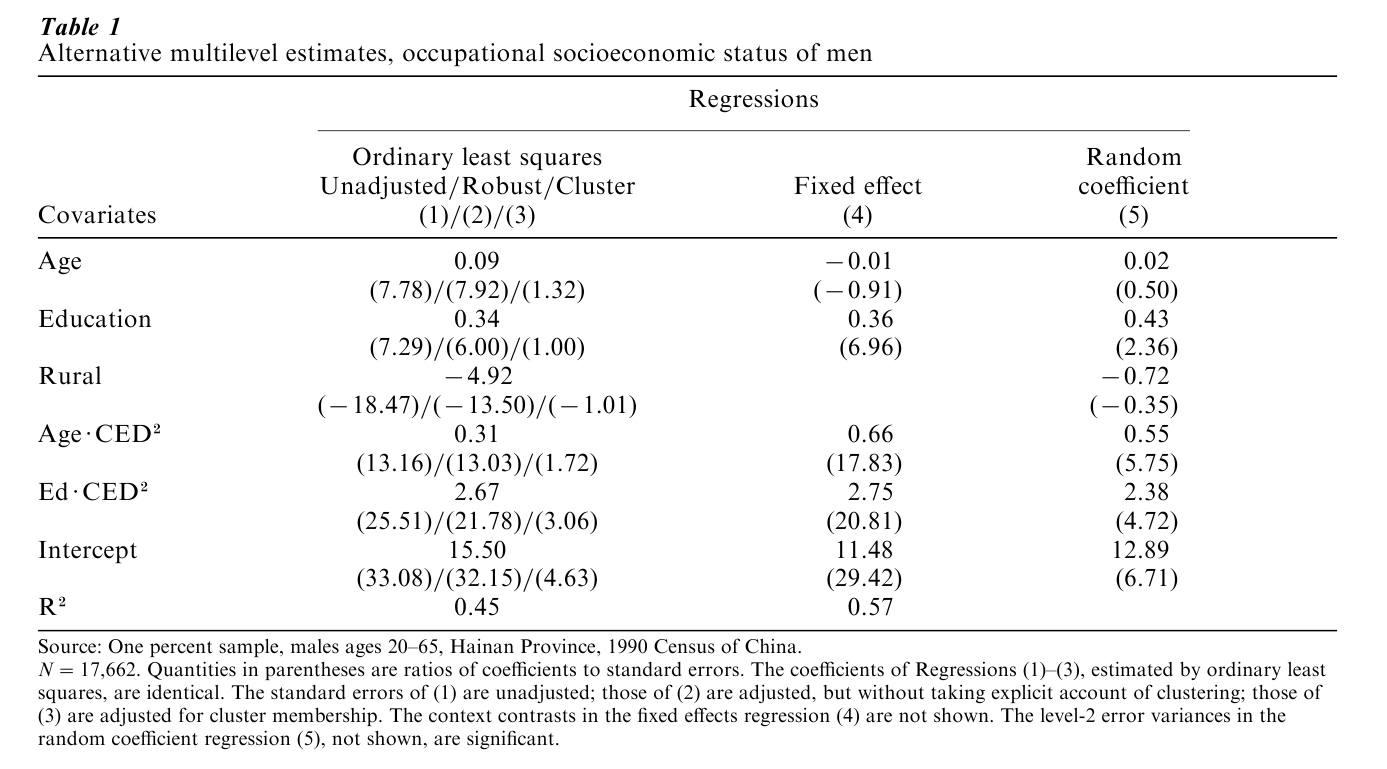
Table 1 reports coefficient estimates and ratios of coefficents to standard errors (‘t-ratios’) for several approaches. Regressions 1–3 are the same ordinary least squares (OLS) regression, differentiated to keep track of the type of standard error. When clustering is ignored, the t-ratios are far larger (regressions 1 and 2). Unstructured adjustment of standard errors makes little difference. Adjusting OLS standard errors for clustering radically reduces the t-ratios (regression 3). The fixed effects coefficients (regression 4) are roughly the same as the OLS coefficients, with larger t-ratios than obtained with the clustering adjustment. Only one term is ‘significant’ when the clustering adjustment is used, whereas three of the four estimable coefficients are highly ‘significant’ in the fixed effects model. The coefficients of the random effects model (regression 5) are comparable with those for the fixed effects model (where present), but the t-ratios are smaller. For those terms present in both the fixed effects and random coefficient models, coefficients are either significant in both models, or not significant in both. In computations not displayed here, the random coefficient specification was computed twice within two different programs, once using maximum likelihood and once using restricted maximum likelihood. There was agreement across programs and methods. Although the basic conclusion is the same for the fixed effects and random coefficient models and differs somewhat from that provided by the clustering adjustment, the variation in coefficient magnitudes and t-ratios across the models is cautionary. Even in the Gaussian case, it can be misleading to estimate a model using only one approach.

6.2 Binary Response Example

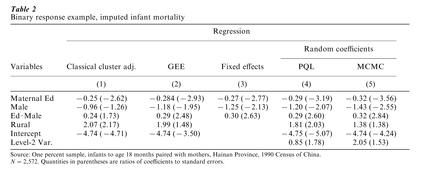
In the binary response example, data from the 1990 Hainan sample are again used. Infants and toddlers born in the 18 months prior to the starting date of the Census enumeration are the level-1 units of observation, and enumeration districts are level-2 observations. The available data do not record child mortality, which has been inferred from maternal information elicited in the Census questionnaire. The response variable is whether an imputed death to a child born after 1988 occurred prior to July 1, 1990. There are 43 imputed deaths out of 2,572 mother–child pairs. A majority of enumeration districts have no imputed deaths. For this reason, only the within-context intercept is treated as random. For ω, the logit of a death within the first 18 months of life, the specification treats the probability of death as a function of maternal years of schooling, the sex of the child, and the interaction between maternal education and sex of child. The intercept is treated as a function of type of place of residence (the same for all residents of an enumeration district) and a random error:

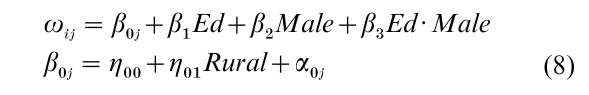
Table 2 presents a selection of regressions based on alternative multilevel approaches and algorithms. Regression 1 is the result of classical maximum likelihood estimation followed by an adjustment for clustering. Using this approach, neither the sex of the child nor the sex–education interaction is ‘significant.’ Using the GEE approach, the coefficient for sex is at the cusp of conventional significance and the sex– education interaction is significant (regression 2). The fixed effects results, using conditional logistic regression, indicate significance for all included terms (regression 3). Penalized quasi-likelihood estimates are provided by regression 4. These are consistent with the fixed effects results for those terms present across the fixed and random effects specifications. Regression 5 presents Bayesian results based on MCMC. The type of place of residence coefficient is smallest and not significant in the Bayesian regression. Application of a clustering adjustment to the GEE results (not shown) also substantially affects conclusions about statistical significance.

It is not unusual to encounter sparse data. This binary response example is perhaps even more cautionary than the Gaussian example. Researchers are not yet routinely able to determine whether convergence is to a local or a global maximum, whether sufficient iterations have been calculated using MCMC, whether all of the assumptions required for a particular method are valid in a given instance, or whether software is performing as intended.

7. Conclusions

Analysis of multilevel data structures using methods that ignore the clustering of observations in the data is unsatisfactory because it can lead to confidence intervals that are too narrow, and to coefficient bias. Random coefficient models—and their specializations and generalizations—are attractive tools for the analysis of multilevel data. When there is selection into contexts, the random coefficient approach is subject to coefficient bias, as it is more generally when there are omitted regressors at any level. The fixed effects approach provides one kind of solution to the omitted variables problem. Instrumental variable estimation offers another. A posterior adjustment to accommodate clustering, applied to the estimated variances of coefficients, is robust but inefficient when the random effects model is correct. Although this adjustment does not require orthogonality between errors and covariates, robust standard errors for biased coefficients are far from universally desirable. For discrete and count responses, marginal models estimated using GEE provide an alternative to random effects models. Marginal models are attractive when there is little interest in within-context estimates, or when the pattern of within-context correlation is not simple. The choice of a multilevel modeling approach is ideally governed by research goals, the study design, and the nature of the data. There is also value in crosschecking results across methods and software.

8. Further Reading

For an introduction to random coefficient models (terminology often used interchangeably with random effects models and hierarchical models), see Snijders and Bosker (1999). The level of exposition in Bryk and Raudenbush (1992) ranges from introductory to advanced, as is also true for Goldstein (1995). The exposition in Longford (1993) is technically demanding. Littell et al. (1996) survey mixed models in general, and include material on hierarchical models. Gilks et al. (1998) and Gelman et al. (1995) are useful for Bayesian random coefficient models. Draper (2002) provides a detailed introduction to random coefficient models from the Bayesian perspective.

Fixed effects modeling is treated in econometrics texts (e.g., Greene 2000), and is often discussed as one approach to the analysis of panel data (Baltagi 1995). For the binary response case, see Pendergast et al. (1996), who provide a review with broad scope. Robust adjustments of standard errors for clustering (e.g., Rogers 1993) are an extension of the methodology of Huber (1967) and White (1980, 1982). The GEE approach is well exposited in Diggle et al. (1994), who provide detailed comparisons with random coefficient and other models. In this same vein, Allison’s (1999) introduction should not be missed. Instrumental variables estimation is a standard subject in econometrics texts (e.g., Greene 2000).

For an illuminating use of random coefficient models in the study of neighborhoods see Sampson et al. (1997). Geronimus and Korenman (1992) use a fixed effects approach in the study of teen pregnancy. Hamilton and Hamilton (1997) use a fixed effects approach in the analysis of surgery outcomes. For the same kind of problem, but using a different data structure, McClellan et al. (1994) employ an instrumental variables approach. Applications of marginal models are found largely in the epidemiological and biomedical literature. Multilevel analysis has long been mainstream in economics, and will soon become so in the rest of the social sciences.

Bibliography:

1. Allison P D 1999 Logistic Regression Using the SAS System. SAS Institute, Cary, NC
2. Baltagi B H 1995 Economic Analysis of Panel Data. Wiley, New York
3. Bryk A S, Raudenbush S W 1992 Hierarchical Linear Models. Sage, Newbury Park, CA
4. Chamberlain G 1980 Analysis of covariance with qualitative data. Review of Economic Studies 47: 225–038
5. Diggle P J, Liang K-Y, Zeger S L 1994 Analysis of Longitudinal Data. Oxford University Press, Oxford, UK
6. Draper D 2002 Bayesian Hierarchical Modeling. SpringerVerlag, New York
7. Gelman A, Carlin J B, Stern H S, Rubin D B 1995 Bayesian Data Analysis. CRC Press, Boca Raton, FL
8. Geronimus A T, Korenman S 1992 The socioeconomic consequences of teen childbearing reconsidered. Quarterly Journal of Economics 107: 1187–214
9. Gilks W R, Richardson S, Spiegelhalter D J 1998 Marko Chain Monte Carlo in Practice. Chapman & Hall, London
10. Goldstein H 1995 Multilevel Statistical Models, 2nd edn. Halstead, New York
11. Goldstein H, Rasbash J, Plewis I, Draper D, Browne W, Yang M, Woodhouse G, Healy M 1998 A User’s Guide to MLwiN. Multilevel Models Project, Institute of Education, University of London, London
12. Greene W H 2000 Econometric Analysis, 4th edn. Prentice-Hall, Upper Saddle River, NJ
13. Hamilton B H, Hamilton V H 1997 Estimating surgical volume—outcome relationships applying survival models: Accounting for frailty and hospital fixed eff Health Economics 6: 383–95
14. Huber P J 1967 The behavior of maximum likelihood estimators under nonstandard conditions. In: LeCam L M, Neyman J (eds.) Proceedings of the Fifth Berkeley Symposium on Mathematical Statistics and Probability. University of California Press, Berkeley, CA, Vol. 1, pp. 221–33
15. Liang, K-Y, Zeger S L 1986 Longitudinal data analysis using generalized linear models. Biometrika 73: 13–22
16. Littell R C, Milliken G A, Stroup W W, Wolfinger R D 1996 SAS System for Mixed Models. SAS Institute, Cary, NC
17. Longford N T 1993 Random Coefficient Models. Oxford University Press, New York
18. McClellan M, McNeil B J, Newhouse J P 1994 Does more intensive treatment of acute myocardial infarction in the elderly reduce mortality? Journal of the American Medical Association 272: 859–66
19. McCullagh P, Nelder J A 1989 Generalized Linear Models. Chapman and Hall, New York
20. Pendergast J F, Gange S J, Newton M A, Lindstrom M J, Palta M, Fisher M R 1996 A survey of methods for analyzing clustered binary response data. International Statistical Review 64: 89–118
21. Raudenbush S, Bryk A, Cheong Y F, Congdon R 2000 HLM 5: Hierarchical Linear and Nonlinear Modeling. Scientific Software International, Lincolnwood, IL
22. Rogers W H 1993 Regression standard errors in clustered samples. Stata Technical Bulletin 13: 19–23
23. Sampson, R J, Raudenbush, S W, Earls F 1997 Neighborhoods and violent crime: A multilevel study of collective effi Science 277: 918–24
24. Snijders T A B, Bosker R 1999 Multilevel Analysis. Sage Publications, London
25. White H 1980 A heteroskedasticity-consistent covariance matrix estimator and a direct test for heteroskedasticity. Econometrica 48: 817–38
26. White H 1982 Maximum likelihood estimation of misspecified models. Econometrica 50: 1–25
27. Zeger S L, Liang K-Y 1986 Longitudinal data analysis for discrete and continuous outcomes. Biometrics 42: 121–30