Instrumental Variables Research Paper

1. The Method Of Instrumental Variables

1.1 Common Problems With Standard Regression Analysis Of Observational Data

In many cases in the social and behavioral sciences, one is interested in a reliable estimate of the causal effect of one variable on another. For example, suppose a mayor is considering increasing the size of the police force; what is the effect of an additional police officer on the crime rate? Or, what is the effect of an additional year of schooling on future earnings? What will happen to economic growth if the central bank raises short-term interest rates by one percentage point? What is the effect of a new medical procedure on health outcomes? These and many other questions require estimates that are causal, in the sense that they are externally valid and can be used to predict the effect of changes in policies or treatments, holding other things constant.

In theory, such causal effects could be estimated by a suitably designed randomized controlled experiment. Very often, however, as in the first three questions, such an experiment could be prohibitively expensive, could be unethical, and/or could have questionable external validity. Even when randomized controlled experiments are available, such as clinical trials of medical procedures, it is of interest to validate the experimental predictions using information on outcomes in the field. Thus, to address such questions empirically typically entails the use of nonexperimental, i.e., observational, data.

Unfortunately, standard regression analysis of observational data can fail to yield reliable estimates of causal effects for many reasons, four of which are particularly salient. First, there could be additional unmeasured effects, leading to ‘omitted variable bias’; for example, the educational attainment of parents is correlated with that of their children, so if parents’ education facilitates learning at home but is unobserved then the correlation between years of school and earnings could overstate the true, causal effect of school on earnings. Second, there might be reverse causality, or ‘simultaneous equations’ bias; for example, more police officers might reduce crime, but cities with higher crime rates might demand more police officers, so standard regression analysis of crime rates on the number of police confounds these two different effects. Third, there could be selection bias, in which those most likely to benefit from a treatment are also most likely to receive it; for example, because ambition is one reason for success both at school and in the labor market, the measured correlation between years of school and earnings could simply reflect the effect of unmeasured ambition. Fourth, standard regression estimates of the causal effect are biased if the regressor is measured with error.

1.2 IV Regression

IV regression provides a way to handle these problems. The main early application of IV methods was for estimating the parameters of a system of linear simultaneous equations, and this remains a good expositional framework. Let y_i denote the outcome variable of interest (say, log future earnings), let Y_i denote the r treatment variables (years of education), let X_i denote K₁ additional observed control variables, and let Z_i denote the K₂ instrumental variables, where these are all observed for observations i=1,…, N. Also let β and γ be unknown parameter vectors, let Φ and Π be matrices of unknown parameters, and let β denote the transpose of β. Suppose that these variables are linearly related as

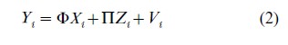
where u_i and V_i are ‘error terms’ that represent additional unobserved effects, measurement error, etc. The coefficient of interest is β; in the schooling example, this is the percentage change in future earnings caused by attending school for an additional year.

In this notation, the four problems listed in the preceding paragraph have a common implication, that the correlation between Y_i and u_i is nonzero, and in consequence the ordinary least squares (OLS) estimator of β will be biased and, in large samples, inconsistent. It is assumed that corr (X_i, u_i) =0; at this level, this assumption can be made without loss of generality, for if this is suspected to be false for some element of X, then it should be listed instead in Y. In the terminology of simultaneous equations theory, y and Y are endogenous variables and X is exogenous.

The key idea of IV methods is that although Y is correlated with u, if Z is uncorrelated with u (that is, if Z is exogenous), then Z can be used to estimate β. Intuitively, part of the variation in Y is endogenous and part is exogenous; IV methods use Z to isolate exogenous variation in Y and thereby to estimate β. More formally, consider the simplest case, in which there is no X in (1) or (2) and which Y and Z are single variables (i.e., K₁= 0 and r=K₂=1). Then cov( y, Z ) =β cov(Y, Z )+cov(u, Z )=β cov(Y, Z ). Thus, β=cov( y, Z )/ cov(Y, Z ). This leads to the IV estimator, β^IV = s_yZ /s_YZ, where s_yZ is the sample covariance between y and Z. Evidently, if these two sample covariances are consistent and if cov(Y, Z) ≠0, then β^IV→β. The availability of the instrument Z thus permits consistent estimation of β.

If more than r instruments are available, it makes sense to use the extra instruments to improve precision. There are, however, many ways to do this, since each subset of r instruments will produce its own estimate of β. The most common way to combine instruments is to use two stage least squares (2SLS). In the first stage, Eqn. (2) is estimated by OLS, producing the predicted values Y. In the second stage, y is regressed against Y and X, yielding the 2SLS estimator β^2SLS. With only one instrument, this reduces to βIV given above. Under Gaussian disturbances, this provides an asymptotically efficient method for weighting the various instruments that is easy to understand and to implement.

1.3 Conditions For Valid Instruments

The question of whether a candidate set of instruments can be used to estimate β is a special case of the more general problem of identification of parameters in multivariate econometric and statistical models. In the context of (1) and (2), when there is a single Y, the requirements for instrument validity are simple. Then a potential instrument Z must satisfy two conditions: (a) Z is uncorrelated with u; and (b) the partial correlation between Y and Z, given X, is nonzero. The first condition states that the instrument is exogenous. The second condition is that the instrument is relevant. Together, these conditions permit using Z to isolate the exogenous variation in Y and thus to identify β. For example, when r=K₂=1 and there are no Xs, if Z satisfies the two conditions then β is identified by the moment condition derived above, β = cov( y, Z)/cov(Y, Z).

When Y is a vector (i.e., r >1), the exogeneity condition (a) remains but the relevance condition (b) is somewhat more complicated. For identification of the independent effects of each Y (all elements of β), a sufficient condition for instrument validity is that the covariance matrix of Z has full rank and that Π has full row rank. Clearly, a necessary condition for Π to have full row rank is that there are at least as many instruments as Ys (K₂≥ r). The number of excess instruments, K₂– r, is referred to as the degree of overidentification of β.

When y is a vector, so that (1) is itself a system of multiple equations, the conditions for identification become intricate. For a rigorous and complete treatment in the linear simultaneous equations framework, see Rothenberg (1971) and Hsiao (1983).

2. IV Estimators And Their Distributions

2.1 Linear Models

In addition to two stage least squares, other estimators are available for IV estimation of a single equation that is linear in the unknown parameters. The leading alternative estimator is the so-called limited information maximum likelihood (LIML) estimator. The LIML estimator minimizes the Anderson–Rubin (1949) statistic,

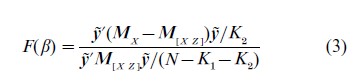
Y=(y₁,… ,y_N) , where y_i= y_i -β´Y_i, and M_X =I X(X´X )⁻¹X´, where X= (X₁, … , X_N) . This can be solved analytically as an eigenvalue problem. Many other single-equation IV estimators have been pro- posed, but these are rarely used in empirical applications; see Hausman (1983) for expressions for the LIML estimator and for a discussion of other estimators.

Under standard assumptions (fixed numbers of regressors and instruments, validity of the instruments, convergence of sample moments to population counterparts, and the ability to apply the central limit theorem), the LIML and 2SLS estimators are asymptotically equivalent and have the same asymptotic norma l distribution. That is, √N(β^LIML-β) and √N(β^2SLS -β) both have asymptotic normal distributions with the same covariance matrix. However, their finite sample distributions differ. There is a large literature on finite sample distributions of these estimators. Because these exact distributions depend on nuisance parameters, such as Π, that are unknown and because few IV statistics are (exactly) pivotal, this literature generally does not provide approximations that are useful in empirical applications. However, some general guidelines do emerge from these studies. Perhaps the most important is that when there are many instruments and/or when Π is small in a suitable sense, LIML tends to exhibit less bias than 2SLS and LIML confidence intervals typically have better coverage rates than 2SLS.

These methods extend naturally to the case that y is a vector and (1) is a system of equations. This entails imposing restrictions on the coefficients in (1) and (2) that are implied by the model, and then using the available instruments to estimate simultaneously all these coefficients with these restrictions imposed. The system analog of 2SLS is three stage least squares, in which all the unknown coefficients are estimated simultaneously using an estimate of the variance-covariance matrix of u obtained from the 2SLS estimates. The system analog of LIML is full information maximum likelihood.

2.2 Nonlinear Models

Many details of the foregoing discussion hinged on the system being linear in the parameters and variables. In many settings, however, theory suggests models that are nonlinear rather than linear. A leading class of examples is consumption-based models of asset prices, in which the equations contain nonlinearities inherited from posited utility functions of representative agents. In such settings, Eqn. (1) is usefully extended and recast to incorporate these nonlinearities. Specifically, suppose that the model at hand implies,

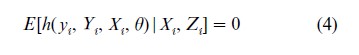
where as before y_i and Y_i are endogenous variables, X_i and Z_i are exogenous variables, and θ is a vector of parameters. For example, in the linear system (1) and (2), (4) is implied by E(u_i |X_i, Z_i)= 0 upon setting h( y_i, Y_i, X_i, θ ) =y_i -β´Y_i -γ´X_i and θ = ( β, γ).

The orthogonality condition (4) corresponds to the first condition for a valid instrument, that Z is exogenous. If in addition Z is relevant, then (4) can be exploited to estimate the unknown parameters θ. The issue of relevance of Z is equivalent to whether θ is identified. The question of identification in nonlinear models is complex and little can be said about global identification at a general level, although conditions for local identification sometimes yield useful insights.

Given a model (4) and a set of instruments, in general a variety of estimators of θ are available. Estimation is typically undertaken by minimization of a quadratic form in h( y_i, Y_i, X_i, θ), times the instruments; 2SLS and LIML estimates obtain as special cases when h is linear. In practice, the choice of the weighting matrix in this quadratic form is important, and if there is serial correlation and/or heteroskedasticity this weighting matrix (and the standard errors) must be computed in a way that accounts for these complications. Such estimators are referred to as generalized method of moments (GMM) estimators. For discussions of identification and estimation in GMM, see Newey and McFadden (1994).

3. A Brief History Of IV Methods

1. Wright (1925) and his father P. Wright (1928) introduced the estimator β^IV (defined in Sect. 1.2) and used it to estimate supply and demand elasticities for butter and flaxseed; this work, however, was neglected (see Goldberger 1972). The development of IV methods in the 1940s stemmed from the attempts of early statisticians and econometricians to solve what appeared to be two different problems: the problem of measurement error in all the variables, and the problem of reverse causality arising in a system of simultaneous equations that describe the macroeconomy. The term ‘instrumental variables’ was first used in print by Reiersøl (1945), who developed IV estimation for the errors in variables problem and extended work by Wald (1940) which, in retrospect, also can be seen as having introduced IV estimation. Concurrently, work by Haavelmo (1944) and the Cowles Commission emphasized likelihood-based methods of analyzing simultaneous equation systems, which implicitly (through identification conditions) entailed the use of instrumental variables; Anderson and Rubin (1949) developed LIML as part of this research program.

An important breakthrough came with the development of 2SLS by Basmann (1957) and Theil (1958), which permitted computationally efficient estimation in single equations with multiple instruments. Sargan (1958) introduced IV estimation for multiple equation systems and Zellner and Theil (1962) developed three stage least squares.

The extension of these methods to nonlinear models was undertaken by Amemiya (1974) (nonlinear 2 SLS) and by Jorgenson and Laffont (1974) (non-linear three stage least squares). The modern formulation of GMM estimation is due to Hansen (1982). GMM constitutes the dominant modern unifying framework for studying the issues of identification, estimation, and inference using IVs.

4. Potential Pitfalls

In practice, inference using IV estimates can be compromised because of failures of the model and/or failures of the asymptotic distribution theory to provide reliable approximations to the finite sample distribution. Much modern work on IV estimation entails finding ways to avoid, or at least to recognize, these pitfalls. This section discusses three specific potentially important pitfalls in linear IV estimation. These problems, as well as additional problems associated with estimation of standard errors, also arise in nonlinear GMM estimation, but their sources and solutions are less well understood in the general nonlinear setting.

4.1 Some Instruments Are Endogenous

If an instrument is endogenous then corr(Z_i, u_i) ≠0, and reflection upon the derivation β^IV and its probability limit in Sect. 1.2 reveals that β^IV is no longer consistent for β. More generally, if at least one instrument is endogenous then the 2SLS and LIML estimators are inconsistent. If at least r instruments are exogenous, however, then it is possible to test the null hypothesis that all instruments are exogenous against the alternative that at least one (but no more than K₂– r) is endogenous. In practice, a researcher might have at least r instruments that he or she firmly believes to be exogenous, but might have some additional instruments which are more questionable.

Testing the null that all the instruments are exogenous entails checking empirically the assumption that the instruments are uncorrelated with u_i. This can be done by regressing the IV residual (estimated by 2SLS or LIML) against Z. The R² of this regression should be zero; if NR² exceeds the desired x²_{K2 −r} critical value, the null hypothesis of joint exogeneity is rejected.

Although this statistic provides a useful diagnostic and rejection suggests that the full instrument list is (jointly) invalid, failure to reject is not necessarily reassuring since the maintained hypothesis is that at least r of the instruments are valid. Moreover, this test can only be implemented if β is overidentified (K₂> r). The hypothesis that at least r instruments are exogenous is both essential and untestable, and thus must be contemplated carefully in IV applications.

4.2 Weak Instruments

The condition for instrument relevance states that Z and Y must have nonzero partial correlation (given X ). In practice, this correlation, while arguably nonzero, is often small, a situation sometimes referred to as the problem of weak instruments. When the instruments are weak, the usual large sample approximations provide a misleading basis for inference: the 2SLS estimator in particular is biased towards the OLS estimator, and asymptotic LIML and 2SLS confidence regions have coverage rates that can differ substantially from the nominal asymptotic confidence level. When r =1, an empirical measure of the strength of the instruments is the F-statistic testing the hypothesis Π =0 in the first stage regression (2). The risk of weak instruments is especially relevant when there are many instruments, for even if some instruments have a large partial correlation with Y, if there are many instruments quite a few of them could be weak so taken together this first-stage F-statistic could be small.

Although no single preferred way to handle weak instruments has yet emerged, one solution is to construct confidence intervals by inverting the Anderson–Rubin statistic (3). This is readily done because F ( β₀) has an asymptotic x²_K2 distribution under the joint null hypothesis that β=β₀ (a fixed vector) and corr(X, u) =corr(Z, u) =0 (the instrument relevance condition is not needed for this result).

4.3 Heterogeneity Of Treatment Effects In Micro Data

Many modern applications of IV are to microdata sets with cross-sectional or panel data, that is, data sets where the observation units are individuals, firms, etc. An important consideration that arises in this context is the role of heterogeneity in interpreting what it is that IV methods measure. To make this concrete, consider a modification of (1) and (2), where for simplicity it is assumed that r=K₂= 1 and the only X is a constant. Suppose, however, that there is heterogeneity both in the responses of each individual to the ‘treatment’ Y and in the influence of the instrument on the level of treatment received. In equations, this can be written as,

where β_i and Π_i vary randomly across individuals. Suppose that the instrument is distributed independently of (u_i, V_i, β_i, Π_i), and technical conditions ensurping convergence of sample moments hold. Then β^2SLS →E [Π_i β_i] /EΠ_i.

Evidently, with heterogeneity of this form 2SLS can be thought of as estimating E [Π_i β_i]/EΠ_i, which differs from the usual estimand β =Eβ_i if β_i and Π_i are correlated. For example, suppose that Π_i =0 for half the population, that Π_i =Π (which is fixed) for the other half, and that the sample is drawn randomly. If β_i differs systematically across the two halves of the population, then 2SLS estimates the mean of βi among that half for which Π_i = Π; this differs from the mean of βi over the full population. More generally, 2SLS can be thought of as estimating a weighted average of the individual treatment effects, where the weights reflect the influence of Z_i on whether the individual receives the treatment. This has been referred to as the ‘local average treatment effect’; see Angrist et al. (1996).

5. Where Do Valid Instruments Come From?

In practice the most difficult aspect of IV estimation is finding instruments that are both exogenous and relevant. There are two main approaches, which reflect two different perspectives on econometric and statistical modeling. The first approach is to use a priori theoretical reasoning to suggest instruments. This is most compelling if the model being estimated is itself derived from a formal theory. An example of this approach is the estimation of intertemporal consumption-based asset pricing models, mentioned in Sect. 2.2 in which previously observed variables are, under the model, uncorrelated with certain future expectational errors. Thus previously observed variables can be used as instruments.

The second approach to constructing instruments, more commonly found in program evaluation studies (broadly defined), is to look for some exogenous source of variation in Y that either derives from true randomization or, in effect, from pseudo-randomization. In randomized experiments in the social sciences, compliance with experimental protocol is usually unenforceable, so a subject’s decision whether to take the treatment introduces selection bias; assignment to treatment, however, can be used as an instrument for receipt of treatment. In nonexperimental settings, this reasoning suggests looking for a variable that plays a role similar to random assignment in a randomized experiment. For example, McClellan, McNeil and Newhouse (1994) investigated the effect of the intensity of treatment (Y ) on mortality after four years ( y) using observational data on elderly Americans who suffered an acute myocardial infarction (heart attack). Standard regression analysis of these data would be subject to selection bias and omitted variables bias, the former because the decision to pursue an intensive treatment depends in part on the severity of the case, the latter because of additional unobserved health characteristics. To avoid these biases, they used as instruments the distance of the patient from hospitals with various degrees of experience treating heart attack patients, for example, the differential distance to a hospital with experience at cardiac catheterization. If distance to such hospitals is distributed randomly across potential heart attack patients, then it is exogenous; if this distance is a factor in the decision whether to move the patient to the distant hospital for intensive treatment, then it is relevant. If both are plausibly true, then 2SLS provides an estimate of the average treatment effect for the marginal patients, where the marginal patients are those for whom the effect of distance on the decision to treat is most important.

From the humble start of estimating how much less butter people will buy if its price rises, IV methods have evolved into a general approach for estimating causal relations throughout the social and behavioral sciences. Because it requires valid and relevant instruments, IV regression is not always an option, and even if it is, the practitioner must be aware of its potential pitfalls. Still, when they can be applied, IV methods constitute perhaps our most powerful weapon against omitted variable bias, reverse causality, selection bias, and errors-in-variables in our efforts to estimate causual relations using observational data. For recent textbook treatments of instrumental variables issues see Hayashi (2000, Chaps. 3 and 4) and Ruud (2000, Chaps. 20–2 and 26).

Bibliography:

1. Amemiya T 1974 The nonlinear two-stage least squares estimator. Journal of Econometrics 2: 105–10
2. Anderson T W, Rubin H 1949 Estimation of the parameters of a single equation in a complete systems of stochastic equations. Annals of Mathematical Statistics 20: 46–63
3. Angrist J D, Imbens G W, Rubin D B 1996 Identification of causal effects using instrumental variables (with discussion). Journal of the American Statistical Association 91: 444–72
4. Basmann, R L 1957 A generalized classical method of linear estimation of coefficients in a structural system of stochastic equations. Annals of Mathematical Statistics 20: 46–63
5. Goldberger A S 1972 Structural equation methods in the social sciences. Econometrica 40: 979–1001
6. Haavelmo T 1944 The probability approach to econometrics. Econometrica 12 (Suppl): 1–118
7. Hansen L P 1982 Large sample properties of generalized method of moments estimators. Econometrica 50: 1029–54
8. Hausman J A 1983 Specification and estimation of simultaneous equation models. In: Grilliches Z, Intrilligator M D (eds.) Handbook of Econometrics. North Holland, Amsterdam, Vol. 1, pp. 391–450
9. Hayashi F 2000 Econometrics. Princeton University Press, Princeton, NJ
10. Hsiao C 1983 Identification. In: Grilliches Z, Intrilligator M D (eds.) Handbook of Econometrics. North Holland, Amsterdam, Vol. 1, pp. 223–83
11. Jorgenson D W, Laffont J 1974 Efficient estimation of nonlinear simultaneous equations with additive disturbances. Annals of Economic and Social Measurement 3: 615–40
12. McClellan M, McNeil B J, Newhouse J P 1994 Does more intensive treatment of acute myocardial infarction in the elderly reduce mortality? Analysis using instrumental variables. Journal of the American Medical Association 272: 859–66
13. Newey W K, McFadden D 1994 Large sample estimation and hypothesis testing. In: Engle R F, McFadden D (eds.) Handbook of Econometrics. North Holland, Amsterdam, Vol. 4, pp. 2113–247
14. Reiersøl O 1945 Confluence analysis by means of instrumental sets of variables. Arki for Mathematik Astronomi och Fysik 32: 1–119
15. Rothenberg T J 1971 Identification in parametric models. Econometrica 39: 577–95
16. Ruud P A 2000 An Introduction to Classical Econometric Theory. Oxford University Press, New York
17. Sargan J D 1958 On the estimation of economic relationships by means of instrumental variables. Journal of the Royal Statistical Society, Series B 21: 91–105
18. Theil H 1958 Economic Forecasts and Policy. North Holland, Amsterdam
19. Wald A 1940 The fitting of straight lines if both variables are subject to error. Annals of Mathematical Statistics 11: 284–300
20. Wright S 1925 Corn and Hog Correlations. US Department of Agriculture Bulletin 1300, January 1925, Washington, DC
21. Wright P G 1928 The Tariff on Animal and Vegetable Oils. Macmillan, New York
22. Zellner A, H Theil 1962 Three-stage least squares: Simultaneous estimation of simultaneous equations. Econometrica 30: 54–78