Scaling in Correspondence Analysis Research Paper

1. Historical Background

Benzecri’s contribution to data analysis in general and to correspondence analysis in particular was not so much in the mathematical theory underlying the methodology as in the strong attention paid to the graphical interpretation of the results and in the broad applicability of the methods to problems in many contexts. His initial interest was in analyzing large sparse matrices of word counts in linguistics, but he soon realized the power of the method in fields as diverse as biology, archeology, physics, and music. The fact that his approach paid so much attention to the visualization of data, to be interpreted with a degree of ingenuity and insight into the substantive problem, fitted perfectly the esprit geometrique of the French and their tradition of visual abstraction and creativity.

Originally working in Rennes in western France, this group consolidated in Paris in the 1970s to become an influential and controversial movement in post-1968 France. In 1973 they published the two fundamental volumes of, L’Analyse des Donnees (Data Analysis), the first on La Classification, that is, unsupervised classification or cluster analysis, and the second on, L’Analyse des Correspondances, or correspondence analysis (Benzecri 1973), as well as from 1977 the journal Les Cahiers de l’Analyse des Donnees, all of which reflect the depth and diversity of Benzecri’s work. For a more complete historical account of the origins of correspondence analysis, see Nishisato (1980), Greenacre (1984), and Gifi (1990).

2. Correspondence Analysis

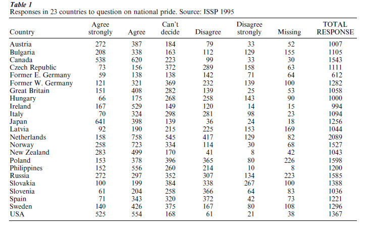
Correspondence analysis (CA) is a variant of principal components analysis (PCA) applicable to categorical data rather than interval-level measurement data. For example, Table 1 is a contingency table obtained fromthe 1995 International Social Survey Program (ISSP) survey on national identity, tabulating responses from 23 countries on the question: ‘How much do you agree/disagree with the statement: Generally (respondent’s country) is a country better than most other countries?’ (For example, Austrians are asked to evaluate the statement: Generally Austria is a country better than most other countries.)

The object of CA is to obtain a graphical display in the form of a spatial map of the rows (countries) and columns (question responses), where the dimensions of the map as well as the specific positions of the row and column points can be interpreted.

The theory of CA can be summarized by the following steps:

(a) Let N be the I ×J table with grand total n and let P = (1/n) N be the correspondence matrix, with grand total equal to 1. CA actually analyzes the correspondence matrix, which is free of the sample size. If N is a contingency table, then P is an observed bivariate discrete distribution.

(b) Let r and c be the vectors of row and columnmsums of P respectively and D_r and D_c diagonal matrices with r and c on the diagonal.

(c) Compute the singular value decomposition of the centred and standardized matrix with general element (p_ij – r_ic_j) / √r_ic_j:

where the singular values are in descending order: α₁ ≥ α₂ ≥ … and U^TU = V^TV = I.

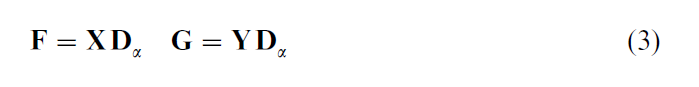
(d) Compute the standard coordinates X and Y:

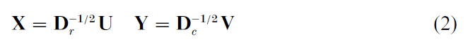
and principal coordinates F and G:

Notice the following:

The results of CA are in the form of a map of points representing the rows and columns with respect to a selected pair of principal axes, corresponding to pairs of columns of the coordinate matrices—usually the first two columns for the first two principal axes. The choice between principal and standard coordinates is described below.

Table 1 Responses in 23 countries to question on national pride. Source: ISSP 1995

The total variance, called inertia, is equal to the sum of squares of the matrix decomposed in (1):

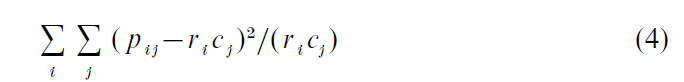
which is the Pearson chi-squared statistic calculated on the original table divided by n.

The squared singular values α₁², α₂²,…, called the principal inertias, decompose the inertia into parts attributable to the respective principal axes, just as in PCA the total variance is decomposed along principal axes.

The most popular type of map, called the symmetric map, uses the first two columns of F for the row coordinates and the first two columns of G for the column coordinates, that is both in principal coordinates as given by (3).

An alternative scaling, which has a more coherent geometric interpretation, but less aesthetic appearance, is the asymmetric map, for example, rows in principal coordinates F and columns in standard coordinates Y in (2) (or vice versa). The choice between a row-principal or column-principal asymmetric map is governed by whether the original table is considered as a set of rows or a set of columns, respectively, when expressed in percentage form.

The positions of the rows and the columns in a map are projections of points, called profiles, from their true positions in high-dimensional space onto a bestfitting lower-dimensional space. A row or column profile is the corresponding row or column of the table divided by its respective total—in the case of a contingency table the profile is a conditional frequency distribution. Each profile is weighted by a mass equal to the value of the corresponding row or column margin, r_i or c_j. The space of the profiles is structured by a weighted Euclidean distance function called the chi-squared distance and the optimal map is obtained by fitting a lower-dimensional space which fits the profiles by weighted least-squares.

Equivalent forms of (4) which show the use of profile, mass, and chi-squared distance are:

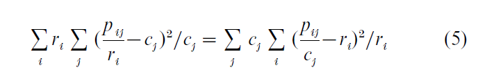
Thus the inertia is a weighted averpage squared distance between the profile vectors (e.g., ij, j = 1,… for a row profile, weighted by the mass r_i) and their respective average (e.g., c_j, j = 1,…, the average row profile), where the distance is of a weighted Euclidean form (e.g., with inverse weighting of the j-th term by c_j).

An equivalent definition of CA is as a pair of classical scaling problems, one for the rows and one for the columns. For example, a square symmetric matrix of chi-squared distances can be calculated between the row profiles, with each point weighted by its respective row mass. Applying classical scaling (also known as principal coordinate analysis, see Scaling: Multidimensional) to this distance matrix, and taking the row masses into account, leads to the row principal coordinates in CA.

The singular value decomposition (SVD) may be written in terms of the standard coordinates in the following equivalent form, for the (i, j)-th element:

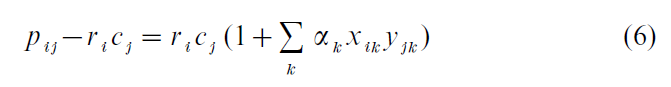
which shows that CA can be considered as a bilinear model. For any particular solution, for example in two dimensions where the first two terms of this decomposition are retained, the residual elements have been minimized by weighted least-squares.

3. Application

The symmetric map of Table 1, with rows and columns in principal coordinates, is given in Fig. 1. Looking at the positions of the question responses first with respect to the first (horizontal) principal axis, they are seen to lie in their substantive order from ‘strongly disagree’ on the left to ‘strongly agree’ on the right, with ‘missing’ on the disagreement side. The scale values of these categories constitute an optimal scale, by which is meant a standardized interval scale for the categorical variable of agreement—disagreement, including the missing value category, which optimally discriminates between the 23 countries, that is which gives maximum between-country variance.

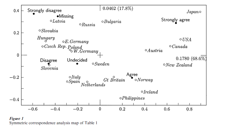
In the two-dimensional map the response category points form a curve known as the ‘horseshoe’ or ‘arch’ which is fairly common for data on an ordinal scale. The second dimension then separates out polarized groups towards the top, or inside the arch, where both extremes of the response scale lie, as well as the missing response in this case.

Turning attention to the countries now, they will line up from left to right in an ordination of agreement induced by the scale values. The five Eastern Bloc countries lie on the left, unfavorable, extreme of the map, with Japan, Canada, USA, and New Zealand at the other, favorable side. The countries generally follow the curved shape as well, but a country such as Bulgaria which lies in a unique position inside the curve is characterized by a relatively high polarization of responses as well as high missing values. Bulgaria’s position in the middle of the first axis contrasts with the position of Great Britain, for example, which is also in the middle but due to responses more in the intermediate categories of the scale rather than a mixture of extreme responses.

The principal inertias are indicated in Fig. 1 at the positive end of each axis and the quality of the display is measured by adding together the percentages of inertia, 68.6 percent + 17.8 percent = 86.4 percent. This means that there is a ‘residual’ of 13.6 percent not depicted in the map, which can only be interpreted by investigating the next dimensions from third onwards. This 13.6 percent is the percentage of inertia minimized in the weighted least-squares solution of CA in two dimensions.

4. Contributions To Inertia

Apart from assessing the quality of the map by the percentages of inertia, other more detailed diagnostics in CA are the so-called contributions to inertia, based on the two decompositions of the total inertia, first by rows and second by columns:

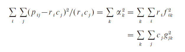
Every row component r_i f²_ik, (respectively, column component c_jg ²_jk ) can be expressed relative to the principal inertia α_k² of the corresponding dimension k, where α_k² is the sum of these components for all the rows (respectively, columns). These relative values provide a diagnostic for deciding which rows (respectively, columns) are important in the determination of the k-th principal axis.

In a similar way, for a fixed row each row component r_i f²_ik (respectively, column component c_jg²_jk for a fixed column) can be expresse d relative to the total ∑_k r_i f²_ik (respectively, ∑_k c_j g²_jk) across all principal axes. These relative values provide a diagnostic for deciding which axes are important in explaining each row or column. These values are analogous to the squared factor loadings in factor analysis, that is, squared correlations between the row or column and the corresponding principal axis or factor.

5. Extensions

Although the primary application of CA is to a two-way contingency table, the method is regularly applied to analyze multiway tables, tables of preferences, ratings, as well as measurement data on ratio or interval-level scales. For multiway tables there are two approaches. The first approach is to convert the table to a flat two-way table which is appropriate to the problem at hand. Thus, if a third variable is introduced into the example above, say ‘sex of respondent,’ then an appropriate way to flatten the three-way table would be to interactively code ‘country’ and ‘sex’ as a new row variable, with 23 × 2 = 46 categories, cross-tabulated against the question responses. For each country there would now be a male and a female point and one could compare sexes and countries in this richer map. This process of interactive coding of the variables can continue as long as the data do not become too fragmented into interactive categories of very low frequency.

Another approach to multiway data, called multiple correspondence analysis (MCA), applies when there are several categorical variables skirting the same issue, often called ‘items.’ MCA is usually defined as the CA algorithm applied to an indicator matrix Z with the rows being the respondents or other sampling units, and the columns being dummy variables for each of the categories of all the variables. The data are zeros and ones, with the ones indicating the chosen categories for each respondent. The resultant map shows each category as a point and, in principle, the position of each respondent as well. Alternatively, one can set up what is called the Burt matrix), B = Z^TZ, the square symmetric table of all two-way cross-tabulations of the variables, including the cross-tabulations of each variable with itself (named after the psychologist Sir Cyril Burt). The Burt matrix is reminiscent of a covariance matrix and the CA of the Burt matrix can be likened to a PCA of a covariance matrix. The analysis of the indicator matrix Z and the Burt matrix B give equivalent standard coordinates of the category points, but slightly different scalings in the principal coordinates since the principal inertias of B are the squares of those of Z.

A variant of MCA called joint correspondence analysis (JCA) avoids the fitting of the tables on the diagonal of the Burt matrix, which is analogous to least-squares factor analysis.

As far as other types of data are concerned, namely rankings, ratings, paired comparisons, ratio-scale, and interval-scale measurements, the key idea is to recode the data in a form which justifies the basic constructs of CA, namely profile, mass, and chi-squared distance. For example, in the analysis of rankings, or preferences, applying the CA algorithm to the original rankings of a set of objects by a sample of subjects is difficult to justify, because there is no reason why weight should be accorded to an object in proportion to its average ranking. A practice called doubling resolves the issue by adding either an ‘anti-object’ for each ranked object or an ‘anti-subject’ for each responding subject, in both cases with rankings in the reverse order. This addition of apparently redundant data leads to CA effectively performing different variants of principal components analysis on the original rankings.

A recent finding by Carroll et al. (1997) is that CA can be applied to a square symmetric matrix of squared distances, transformed by subtracting each squared distance from a constant which is substantially larger than the largest squared distance in the table. This yields a solution which approximates the classical scaling solution of the distance matrix.

All these extensions of CA conform closely to Benzecri’s original conception of CA as a universal technique for exploring many different types of data through operations such as doubling or other judicious transformations of the data.

The latest developments on the subject, including discussions of sampling properties of CA solutions and a comprehensive reference list, may be found in the volumes edited by Greenacre and Blasius (1994) and Blasius and Greenacre (1998).

Bibliography:

1. Benzecri J-P 1973 L’Analyse des Donnees Vol I: La Classification, Vol. II: L’Analyse des Correspondances. Dunod, Paris
2. Blasius J, Greenacre M J 1998 Visualization of Categorical Data. Academic Press, San Diego, CA
3. Carroll J D, Kumbasar E, Romney A K 1997 An equivalence relation between correspondence analysis and classical metric multidimensional scaling for the recovery of Euclidean distances. British Journal of Mathematical and Statistical Psychology 50: 81–92
4. Gifi A 1990 Nonlinear Multivariate Analysis. Wiley, Chichester, UK
5. Greenacre M J 1984 Theory and Applications of Correspondence Analysis. Academic Press, London
6. Greenacre M J 1993 Correspondence Analysis in Practice. Academic Press, London
7. Greenacre M J, Blasius J 1994 Correspondence Analysis in the Social Sciences. Academic Press, London
8. International Social Survey Program (ISSP) 1995 Survey on National Identity. Data set ZA 2880, Zentralarchiv fur Empirische Sozialforschung. University of Cologne
9. Lebart L, Morineau A, Warwick K 1984 Multivariate Descriptive Statistical Analysis. Wiley, Chichester, UK
10. Nishisato S 1980 Analysis of Categorical Data: Dual Scaling and its Applications. University of Toronto Press, Toronto, Canada