Screening And Selection Research Paper

2. Basic Concepts

The purpose of a screening test is to determine whether a person or object is a member of a particular class, C or its complement, C -. The test result indicating that the person is in C will be denoted by S and a result indicating non-membership by S -. The accuracy of a test is described by two probabilities:

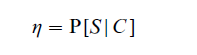
being the probability that someone in C is correctly classified, or the sensitivity of the test; and

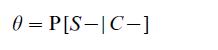
being the probability that someone not in C is correctly classified, or the specificity of the test. Given the prevalence, π = P(C ), of the trait in the population screened, from Bayes’ theorem it follows that the predictive value of a positive test (PVP) is

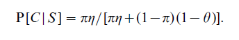
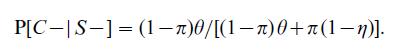
Similarly, the predictive value of a negative test is

In the first two sections, we will assume that the accuracy rates and the prevalence are known. When they are estimated from data, appropriate sampling errors for them and the PVP are given in Gastwirth (1987).

For illustration, consider an early test for HIV, having a sensitivity of 0.98 and a specificity of 0.93, applied in two populations. The first has a very low prevalence, 1.0 × 10⁻³ of the infection while the second has a prevalence of 0.25. From Eqn. (1), the PVP in the first population equals 0.0138, i.e., only about one-and-one-half percent of individuals classified as infected would actually be so. Nearly 99 percent would be false positives. Notice that if the fraction of positives, expected to be 0.0797, in the screened data were used to estimate prevalence, a severe overestimate would result. Adjusting for the error rates yields an accurate estimate. In the higher prevalence group, the PVP is 0.8235, indicating that the test could be useful in identifying individuals. Currently-used tests have accuracy rates greater than 0.99, but even these still have a PVP less than 0.5 when applied to a low prevalence population. A comprehensive discussion is given in Brookmeyer and Gail (1994).

The role of the prevalence, also called the base rate, of the trait in the screened population and how well people understand its effect has been the subject of substantial research, recently reviewed by Koehler (1996). An interesting consequence is that when steps are taken to reduce the prevalence of the trait prior to screening, the PVP declines and the fraction of false positives increases. Thus, when high-risk donors are encouraged to defer or when background checks eliminate a sizeable fraction of unsuitable applicants prior to their being subjected to polygraph testing the fraction of classified positives who are truly positive is small.

In many applications screening tests yield data that are ordinal or essentially continuous, e.g., scores on psychological tests or the concentration of HIV antibodies. Any value, t, can be used as a cut-off point to delineate between individuals with the trait and ‘normal.’ Each t generates a corresponding sensitivity and specificity for the test and the user must then incorporate the relative costs of the two different errors and the likely prevalence of the trait in the population being screened to select the cut off. The receiver operating characteristic (ROC) curve displays the trade-off between the sensitivity and specificity defined by various choices of t and also yields a method for comparing two or more screening tests.

To define the ROC curve, assume that the distribution of the measured variable (test score or physical quantity) is F(x) for the ‘normal’ members of the population but is G(x) for those with the trait. The corresponding density functions are f(x) and g(x) respectively and g(x) will be shifted (to the right (left) if large (small) scores indicate the trait) of f (x) for a good screening test. Often one fixes the probability (α = 1 – y θ or one minus the specificity) of classifying a person without the characteristic as having it at a small value. Then t is determined from the equation F (t) = 1 – θ. The sensitivity, η, of the test is 1 – G(t ). The ROC curve plots η against 1 – θ. A perfect test would have η = 1 so the closer the ROC is to the upper left corner in Fig. 1, the better the screening test. In Fig. 1 we assume f is a normal density with mean 0 and variance 1 while g₁ is normal with mean 1 and the same variance. For comparison we also graphed the ROC for a second test, which has a density g₂ with mean 2 and variance 1. Notice that the ROC curve for the second test is closer to the left corner (0,1) than that of the first test.

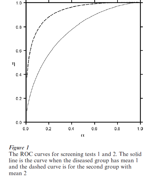
A summary measure (Campbell 1994), which is useful in comparing two screening tests is the area, A, under the ROC. The closer A is to its maximum value of 1.0, the better the test is. In Fig. 1, the areas under the ROC curves for the two tests are 0.761 and 0.922, respectively. Thus, the areas reflect the fact that the ROC curve for the second test is closer to what a ‘perfect’ test would be. This area equals the probability a randomly chosen individual will have a higher score on the screening test than a normal one. This probability is the expected value of the Mann–Whitney form of the Wilcoxon test for comparing two distributions and methods for estimating it are in standard non-parametric statistics texts.

Non-parametric methods for estimating the entire ROC curve are given by Wieand et al. (1989) and Hilgers (1991) obtained distribution-free confidence bounds for it. Campbell (1994) uses the confidence bounds on F and G to construct a joint confidence interval for the sensitivity and one minus the specificity in addition to proposing alternative confidence bounds for the ROC itself. Hseih and Turnbull (1996) determine the value of t that maximizes the sum of sensitivity and specificity. Their approach can be extended to maximizing weighted average of the two accuracy rates, suggested by Gail and Green (1976). Wieand et al. (1989) also developed related statistics focusing on the portion of the ROC lying above a region, α₁ and α₃ so the analysis can be confined to values of specificity that are practically useful. Greenhouse and Mantel (1950) determine the sample sizes needed to test whether both the specificity and sensitivity of a test exceed pre-specified values.

The area A under the ROC can also be estimated using parametric distributions for the densities f and g. References to this literature and an alternative approach using smoothed histograms to estimate the densities is developed in Zou et al. (1997). They also consider estimating the partial area over the important region determined by two appropriate small values of α.

The tests used to select employees need to be reliable and valid. Reliability means that replicate values are consistent while validity means that the test measures what it should, e.g., successful academic performance. Validity is often assessed by the correlation between the test score (X ) and subsequent performance (Y ). Often X and Y can be regarded as jointly normal random variables, especially as monotone transformations of the raw scores can be used in place of them. If a passing score on the screening or pre-employment test is defined as X ≥ t and successful performance is defined as Y ≥ d, then the sensitivity of the test is P[X > t|Y > d ], the specificity is P[X < t |Y < d ] and the prevalence of the trait is P[Y > d ] in the population of potential applicants. Hence, the aptitude and related tests can be viewed from the general screening test paradigm.

When the test and performance scores are scaled to have a standard bivariate normal distribution, both the sensitivity and specificity increase with the correlation, ρ. For example, suppose one desired to obtain employees in the upper half of the performance distribution and used a cut-off score, t, of one-standard deviation above the mean on the test (X ). When ρ = 0.3, the sensitivity is 0.217 while the specificity is 0.899. If ρ = 0.5, the sensitivity is 0.255 and the specificity is 0.937. The use of a high cut-off score eliminates the less able applicants but also disqualifies a majority of applicants who are in the upper half of the performance distribution. Reducing the cut-off score to one-half a standard deviation above the average raises the sensitivities to 0.394 and 0.454 for the two values of ρ but lowers the corresponding specificities to 0.777 and 0.837. This trade-off is a general phenomenon as seen in the ROC curves.

3. The Importance Of The Context In Interpreting The Results Of Screening Tests

In medical and psychological applications, an individual who tests positive for a disease or condition on a screening test will be given a more accurate confirmatory test or intensive interview. The cost of a ‘false positive’ screening result on a medical exam is often considered very small relative to a ‘false negative,’ which could lead to the failure of suitable treatment to be given in a timely fashion. A false positive result presumably would be identified in a subsequent more detailed exam. Similarly, when government agencies give employees in safety or security sensitive jobs a polygraph test, the loss of potentially productive employee due to a false positive was deemed much less than the risk of hiring an employee who would might be a risk to the public or a security risk.

One can formalize the issue by including the costs of various errors and the prevalence, π, of the trait in the population being screened in determining the cut-off value of the screening test. Then the expected cost, which weights the probability of each type of error by its cost is given by

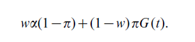
Here the relative costs of a false positive (negative) are w and 1 – w, respectively and as before t = F⁻¹ (1 – α). The choice of cut-off value, t_o, minimizing the expected cost satisfies:

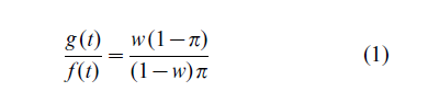
Whenever the ratio, g: f, of the density functions is a monotone function the previous equation yields an optimum cut-off point, t_o, which depends on the costs and prevalence of the trait. Note that for any value of π, the greater the cost of a false positive, the larger will be the optimum value, t_o. This reflects the fact that the specificity needs to be high in order to keep the false positive rate low.

Although the relative costs of the two types of error are not always easy to obtain and the prevalence may only be approximately known, Eqn. (1) may aid in choosing the critical value. In practice, one should also assess the effect slight changes in the costs and assumed prevalence have on the choice of the cut-off value.

The choice of t that satisfies condition (1) may not be optimal if one desires to estimate the prevalence of the trait in a population rather than classifying individuals. Yanagawa and Tokudome (1990) deter- mine t when the objective is to minimize the relative absolute error of the estimator of prevalence on the basis of the screening test results.

The HIV/AIDS epidemic raised questions about the standard assumptions about the relative costs of the two types of error. A ‘false positive’ classification would not only mean that a well individual would worry until the results of the confirmatory test were completed, they also might have social and economic consequences if friends or their employer learned of the result.

Similar problems arise in screening blood donors and in studies concerning the association of genetic markers and serious diseases. Recall that the vast majority of donors or volunteers for genetic studies are doing a public service and are being screened to protect others or advance knowledge. If a donation tests positive, clearly it should not be used for transfusion. Should a screened-positive donor be informed of their status? Because the prevalence of infected donors is very small, the PVP is quite low so that most of the donors screened positive are ‘false.’ Thus, blood banks typically do not inform them and rely on approaches to encourage donors from highrisk groups to exclude themselves from the donor pool (Nusbacher et al. 1986). Similarly, in a study (Hartge et al. 1998) of the prevalence of mutations in two genes that have been linked to cancer the study participants were not notified of their results.

The screening test paradigm is useful in evaluating tests used to select employees. The utility of a test depends on the costs associated with administering the test and the costs associated with the two types of error. Traditionally, employers focused on the costs of a false positive, hiring an employee who does not perform well, such as termination costs, and the possible loss of customers. The costs of a false negative are more difficult to estimate.

The civil-rights law, which was designed to open job opportunities to minorities, emphasized the importance of using appropriate tests, i.e., tests that selected better workers. Employers need to check whether the tests or job requirements (e.g., possession of a high school diploma) have a disparate impact upon a legally protected group. When they exclude a significantly greater fraction of minority members than majority ones, the employer needs to validate it, i.e., show it is predictive of on the job performance. Arvey (1979) and Paetzold and Willborn (1994) discuss these issues.

4. Estimating The Accuracy Of The Screening Tests

So far, we have assumed that we can estimate the accuracy of the screening tests on samples from two populations where the true status of the individuals is known with certainty. In practice, this is often not the case and can lead to biased estimates of the sensitivity and specificity of a screening test, as some of the individuals believed to be normal have the trait, and vice versa.

If one has samples from only one population to which to apply both the screening and confirmatory test, then one cannot estimate the accuracy rates. The data would be organized into a 2 × 2 table, with four cells, only three of which are independent. There are five parameters, however, the two accuracy rates of the two tests plus the prevalence of the trait in the population. In some situations, the prevalence of the trait may vary amongst sub-populations. If one can find two such sub-populations and if the accuracy rates of both tests are the same in both of those subpopulations, then one has two 2 × 2 tables with six independent cells, with which to estimate six parameters. Then estimation can then be carried out (Hui and Walter 1980).

This approach assumes that the two tests are conditionally independent given the true status of the individual. When this assumption is not satisfied, Vacek (1985) showed that the estimates of sensitivity and specificity of the tests are biased. This topic is an active area of research, recently reviewed by Hui and Zhou (1998). A variety of latent-class models have been developed that relax the assumption of conditional independence (see Faraone and Tsuang 1994 and Yang and Becker 1997 and the literature they cite).

5. Applications And Future Concerns

Historically screening tests were used to identify individuals with a disease or trait, e.g., as a first stage in diagnosing medical or psychological conditions or select students or employees. They are being increasingly used, often in conjunction with a second, confirmatory test, in prevalence surveys for public health planning. The techniques developed are often applicable, with suitable modifications, to social science surveys.

Some examples of prevalence surveys illustrate their utility. Katz et al. (1995) compared two instruments for determining the presence of psychiatric disorders in part to assess the needs for psychiatric care in the community and the available services. They found that increasing the original cut-off score yielded higher specificity without a substantial loss of sensitivity. Similar studies were carried out in Holland by Hodiamont et al. (1987) who found a lower prevalence (7.5 percent) than the 16 percent estimate in York. The two studies, however, used different classification systems illustrating that one needs to carefully examine the methodology underlying various surveys before making international comparisons. Gupta et al. (1997) used several criteria based on the results of an EKG and an individual’s medical history to estimate the prevalence of heart disease in India.

Often one has prior knowledge of the prevalence of a trait in a population, especially if one is screening similar populations on a regular basis, as would be employers, medical plans, or blood centers. Bayesian methods incorporate this background information and can yield more accurate estimates (see Geisser 1993, and Johnson, Gastwirth and Pearson 2001). A cost-effective approach is to use an inexpensive screen at a first stage and retest the positives with a more definitive test. Bayesian methodology for such studies was developed by Erkanli et al. (1997).

The problem of misclassification arises often in questionnaire surveys. Laurikka et al. (1995) estimated the sensitivity and specificity of self-reporting of varicose veins. While both measures were greater than 0.90, the specificity was lower (0.83) for individuals with a family history than those with negative histories. Sorenson (1998) observed that often self-reports are accepted as true and found that the potential misclassification could lead to noticeable (10 percent) errors in estimated mortality rates. The distortion misclassification errors can have on estimates of low prevalence traits because of the high fraction of false positive classifications, was illustrated in the earlier discussion of screening tests for HIV/AIDS. Hemenway (1997) applies these concepts to demonstrate that surveys typically overestimate rare events; in particular the self-defense uses of guns. Thus it is essential to incorporate the accuracy rates into the prevalence estimate (Hilden 1979, Gastwirth 1987, Rahme and Joseph 1998).

Sinclair and Gastwirth (1994) utilized the HuiWalter paradigm to assess the accuracy of both the original and re-interview (by supervisors) classifications in labor force surveys. In its evaluation, the Census Bureau assumes that the re-interview data are correct; however, those authors found that both interviews had similar accuracy rates. In situations where one can obtain three or more classifications, all the parameters are identifiable (Walter and Irwig 1988) Gastwirth and Sinclair (1998) utilized this feature of the screening test approach to suggest an alternative design for judge–jury agreement studies that hAdvanother expert, e.g., law professor or retired judge, assess the evidence.

6. Conclusion

Many selection or classification problems can be viewed from the screening test paradigm. The context of the application determines the relative costs of a misclassification or erroneous identification. In criminal trials, society has decided that the cost of an erroneous conviction far outweighs the cost of an erroneous acquittal. While, in testing job applicants, the cost of not hiring a competent worker is not as serious. The two types of error vary with the threshold or cut-off value and the accuracy rates corresponding to these choices is summarized by the ROC curve.

There is a burgeoning literature in this area as researchers are incorporating relevant covariates, e.g., prior health status or educational background into the classification procedures. Recent issues of Biometrics and Multivariate Behavioral Research, Psychometrika and Applied Psychological Measurement as well as the medical journals cited in the paper contain a variety of articles presenting new techniques and applications of them to the problems discussed.

Bibliography:

1. Arvey R D 1979 Fairness in Selecting Employees. AddisonWesley, Reading, MA
2. Brookmeyer R, Gail M H 1994 AIDS Epidemiology: A Quantitative Approach. Oxford University Press, New York
3. Campbell G 1994 Advances in statistical methodology for the evaluation of diagnostic and laboratory tests. Statistics in Medicine 13: 499–508
4. Erkanli A, Soyer R, Stangl D 1997 Bayesian inference in two-phase prevalence studies. Statistics in Medicine 16: 1121–33
5. Faraone S V, Tsuang M T 1994 Measuring diagnostic accuracy in the absence of a gold standard. American Journal of Psychiatry 151: 650–7
6. Gail M H, Green S B 1976 A generalization of the one-sided two-sample Kolmogorov–Smirnov statistic for evaluating diagnostic tests. Biometrics 32: 561–70
7. Gastwirth J L 1987 The statistical precision of medical screening procedures: Application to polygraph and AIDS antibodies test data (with discussion). Statistical Science 2: 213–38
8. Gastwirth J L, Sinclair M D 1998 Diagnostic test methodology in the design and analysis of judge–jury agreement studies. Jurimetrics Journal 39: 59–78
9. Geisser S 1993 Predictive Inference. Chapman and Hall, London
10. Greenhouse S W, Mantel N 1950 The evaluation of diagnostic tests. Biometrics 16: 399–412
11. Gupta R, Prakash H, Gupta V P, Gupta K D 1997 Prevalence and determinants of coronary heart disease in a rural population of India. Journal of Clinical Epidemiology 50: 203–9
12. Hartge P, Struewing J P, Wacholder S, Brody L C, Tucker M A 1999 The prevalence of common BRCA1 and BRCA2 mutations among Ashkenazi jews. American Journal of Human Genetics 64: 963–70
13. Hemenway D 1997 The myth of millions of annual self-defense gun uses: A case study of survey overestimates of rare events. Chance 10: 6–10
14. Hilden J 1979 A further comment on ‘Estimating prevalence from the results of a screening test.’ American Journal of Epidemiology 109: 721–2
15. Hilgers R A 1991 Distribution-free confidence bounds for ROC curves. Methods and Information Medicine 30: 96–101
16. Hodiamont P, Peer N, Syben N 1987 Epidemiological aspects of psychiatric disorder in a Dutch health area. Psychological Medicine 17: 495–505
17. Hseih F S, Turnbull B W 1996 Nonparametric methods for evaluating diagnostic tests. Statistics Sinica 6: 47–62
18. Hui S L, Walter S D 1980 Estimating the error rates of diagnostic tests. Biometrics 36: 167–71
19. Hui S L, Zhou X H 1998 Evaluation of diagnostic tests without gold standards. Statistical Methods in Medical Research 7: 354–70
20. Johnson W O, Gastwirth J L, Pearson L M 2001 Screening without a gold standard: The Hui–Walter paradigm revisited. American Journal of Epidemiology 153: 921–4
21. Katz R, Stephen J, Shaw B F, Matthew A, Newman F, Rosenbluth M 1995 The East York health needs study— Prevalence of DSM-III-R psychiatric disorder in a sample of Canadian women. British Journal of Psychiatry 166: 100–6
22. Koehler J J 1996 The base rate fallacy reconsidered: descriptive, normative and methodological challenges (with discussion). Behavioral and Brain Sciences 19: 1–53
23. Laurikka J, Laara E, Sisto T, Tarkka M, Auvinen O, Hakama M 1995 Misclassification in a questionnaire survey of varicose veins. Journal of Clinical Epidemiology 48: 1175–8
24. Nusbacher J, Chiavetta J, Naiman R, Buchner B, Scalia V, Horst R 1986 Evaluation of a confidential method of excluding blood donors exposed to human immunodeficiency virus. Transfusion 26: 539–41
25. Paetzold R, Willborn S 1994 Statistical Proof of Discrimination. Shepard’s McGraw Hill, Colorado Springs, CO
26. Rahme E, Joseph L 1998 Estimating the prevalence of a rare disease: adjusted maximum likelihood. The Statistician 47: 149–58
27. Sinclair M D, Gastwirth J L 1994 On procedures for evaluating the effectiveness of reinterview survey methods: Application to labor force data. Journal of American Statistical Assn 91: 961–9
28. Sorenson S B 1998 Identifying Hispanics in existing databases. Evaluation Review 22: 520–34
29. Vacek P M 1985 The effect of conditional dependence on the evaluation of diagnostic tests. Biometrics 41: 959–68
30. Walter S D, Irwig L M 1988 Estimation of test error rates, disease prevalence and relative risk from misclassified data: A review. Journal of Clinical Epidemiology 41: 923–37
31. Wieand S, Gail M H, James B R, James K 1989 A family of nonparametric statistics for comparing diagnostic markers with paired or unpaired data. Biometrika 76: 585–92
32. Yanagawa T, Tokudome S 1990 Use of screening tests to assess cancer risk and to estimate the risk of adult T-cell leukemia lymphoma. Environmental Health Perspectives 87: 77–82
33. Yang I, Becker M P 1997 Latent variable modeling of diagnostic accuracy. Biometrics 52: 948–58
34. Zou K H, Hall W J, Shapiro D E 1997 Smooth non-parametric receiver operating characteristic (ROC) curves for continuous diagnostic tests. Statistics in Medicine 16: 214–56