Random Numbers Research Paper

1. Random Number Generators

The words random number actually refer to a poorly defined concept. Formally speaking, one can argue that no number is more random than any other. If a fair dice is thrown eight times, for example, the sequences of outcomes 22222222 and 26142363 have exactly the same chance of occurring, on what basis could the second one be declared more random than the first?

A more precisely defined concept is that of independent random variables. This is a pure mathematical abstraction, which is nevertheless convenient for modeling real-life situations. The outcomes of successive throws of a fair dice, for instance, can be modeled as a sequence of independent random variables uniformly distributed over the set of integers from 1 to 6, i.e., where each of these integers has the probability 1/6 for each outcome, independently of the other outcomes. This is an abstract concept because no absolutely perfect dice exists in the real world.

An RNG is a computer program whose aim is to imitate or simulate the typical behavior of a sequence of independent random variables. Such a program is usually purely deterministic: if started at different times or on different computers with the same initial state of its internal data, i.e., with the same seed, the sequence of numbers produced by the RNG will be exactly the same.

When constructing an RNG to simulate a dice, for example, the aim is that the statistical properties of the sequence of outcomes be representative of what should be expected from an idealized dice. In particular, each number should appear with a frequency near 1/6 in the long run, each pair of successive numbers should appear with a frequency near 1/36, each triplet should appear with a frequency near 1/216, and so on. This would guarantee not only that the virtual dice is unbiased, but also that the successive outcomes are uncorrelated.

However, practical RNGs use a finite amount of memory. The number of states that they can take is finite, and so is the total number of possible streams of successive output values they can produce, from all possible initial states.

Mathematically, an RNG can be defined (see L’Ecuyer 1994) as a structure (S, µ, f, U, g), where S is a finite set of states; µ is a probability distribution on S used to select the initial state (or seed) s ; the mapping f: S → S is the transition function; U is a finite set of output symbols; and g: S → U is the output function.

The state evolves according to the recurrence s_n = f (s_n−1), for n ≥ 1. The output at step n is u_n = g(s_n) ϵ U. These u_n are the so-called random numbers produced by the RNG. Because S is finite, the generator will eventually return to a state already visited (i.e., s_i+j = s_i for some i ≥ 0 and j ≥ 0). Then, s_n+j = s_n and u_n+j = u_n for all n ≥ i. The smallest j > 0 for which this happens is called the period length ρ. It cannot exceed the cardinality of S. In particular, if b bits are used to represent the state, then ρ ≤ 2^b. Good RNGs are designed so that their period length is close to that upper bound.

Choosing s₀ from a uniform initial distribution µ can be crudely approximated by using external randomness such as picking balls from a box or throwing a real dice. The RNG can then be viewed as an extensor of randomness, stretching a short random seed into a long stream of random-looking numbers.

2. Randomness From Physical Devices

Why use a deterministic computer algorithm instead of a truly random mechanism for generating random numbers? Simply calling up a system’s function from a program is certainly more convenient than throwing dice or picking balls from a box and entering the corresponding numbers on a computer’s keyboard, especially when thousands (often millions or even billions) of random numbers are needed for a computer experiment.

Attempts have been made at constructing RNGs from physical devices such as noise diodes, gamma-ray counters, and so on, but these remain largely impractical and unreliable, because they are cumbersome, and because it is generally not true that the successive numbers they produce are independent and uniformly distributed. If one insists on getting away from a purely deterministic algorithm, a sensible compromise is to combine the output of a well-designed RNG with some physical noise, e.g., via bitwise exclusive-or.

3. Quality Criteria

Assume, for the following, that the generator’s purpose is to simulate i.i.d. U [0,1] random variables. The goal is that one cannot easily distinguish between the output sequence of the RNG and a sequence of i.i.d. U [0,1] random variables. That is, the RNG should behave according to the null hypothesis H₀: ‘The u_n are i.i.d. U [0,1],’ which means that for each t, the vector (u₀, …, u_t−1) is uniformally distributed over the t-dimensional unit cube [0.1]^t. Clearly, H₀ cannot be exactly true, because these vectors always take their values only from the finite set

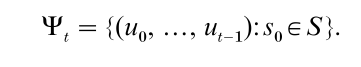
If s₀ is random, Ψ_t can be viewed as the sample space from which the output vectors are taken. The idea, then, is to require that Ψ_t be very evenly distributed over the unit cube, so that H₀ be approximately true for practical purposes. A huge state set S and a very large period length ρ are necessary requirements, but they are not sufficient; good uniformity of the Ψ_t is also needed. When several t-dimensional vectors are produced by an RNG by taking non-overlapping blocks of t output values, this can be viewed in a way as picking points at random from Ψ_t, without replacement.

It remains to agree on a computable figure of merit that measures the evenness of the distribution, and to construct specific RNGs having a good figure of merit in all dimensions t up to some preset number t₁ (because computing the figure of merit for all t up to infinity is infeasible in general). Several measures of discrepancy between the empirical distribution of a point set Ψ_t and the uniform distribution over [0, 1]^t were proposed and studied in the last few decades of the twentieth century (Niederreiter 1992, Hellekalek and Larcher 1998). These measures can be used to define figures of merit for RNGs. A very important criterion in choosing such a measure is the ability to compute it efficiently, and this depends on the mathematical structure of Ψ_t. For this reason, it is customary to use different figures of merit (i.e., different measures of discrepancy) for analyzing different classes of RNGs. Some would argue that Ψ_t should look like a typical set of random points over the unit cube instead of being too evenly distributed. That it should have a chaotic structure, not a regular one. However, chaotic structures are hard to analyze mathematically. It is probably safer to select RNG classes for which the structure of Ψ_t can be analyzed and understood, even if this implies more regularity, rather than selecting an RNG with a chaotic but poorly understood structure.

For a concrete illustration, consider the two linear recurrences

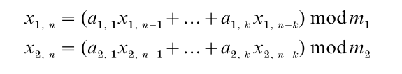
where k, the m_j’s, and the a_{i, j}’s are fixed integers, ‘mod m_j’ means the remainder of the integer division by m_j, and the output function

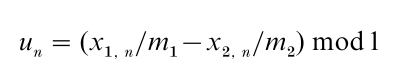
This RNG is a combined linear multiple recursive generator (L’Ecuyer 1999a). Its state at step n is the 2k-dimensional vector

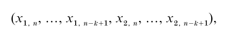
whose first k components are in {0, 1, …, m₁ – 1} and last k components are in {0, 1, …, m₂ – 1}. There are thus (m₁m₂)³ different states and it can be proved that Ψ_k is the set of all k-dimensional vectors with coordinates in {0, 1/m, …, (m-1)/m}, where m=m₁m₂. This implies, if m is large, that for each t ≤ k, the t-dimensional cube [0,1]^t is evenly covered by Ψ_t. For t > k, it turns out that in this case, Ψ_t has a regular lattice structure (Knuth 1998, L’Ecuyer 1998), so that all its points are contained in a series of equidistant parallel hyperplanes, say at a distance d_t apart. To obtain a good coverage of the unit cube, d_t must be as small as possible, and this value can be used as a selection criterion.

L’Ecuyer (1999a) recommends a concrete implementation of the is RNG with the parameter values: k = 3, m₁ = 2³² – 209, (a₁₁, a₁₂, a₁₃) = (0, 1403580, – 810728), m₂ = 2³² – 22853, and (a₁₁, a₁₂, a₁₃) = (527612, 0, – 1370589) . This RNG has two main cycles of length ρ ≈ 2¹⁹¹ each (the total number of states is approximately 2¹⁹²). Its lattice structure has been analyzed in up to t = 48 dimensions and was found to be excellent, in the sense that d_t is not far from the smallest possible value that can be achieved for an arbitrary lattice with (m₁m₂)³ points per unit of volume. These parameters were found by an extensive computer search.

For a second example, consider the linear congruential generator (LCG) defined by the recurrence x_n = ax_n−1 mod m and output function u_n = x_n /m. This type of RNG is widely used and is still the default generator in several (perhaps the majority of) software systems. With the popular choice of m = 2³¹ – 1 and a = 16807 for the parameters, the period length is 2³¹ – 2, which is now deemed much too small for serious applications (Law and Kelton 2000, L’Ecuyer 1998). This RNG also has a lattice structure similar to the previous one, except that the distances d_t are much larger, and this can easily show up in simulation results (Hellekalek and Larcher 1998, L’Ecuyer and Simard 2000). Small LCGs of this type should be discarded.

Another way of assessing the uniformity is in terms of the leading bits of the successive output values, as follows. Suppose that S (and Ψ_t) has cardinality 2^e. There are tl possibilities for the l most significant bits of t successive output values u_n, …, u_n+t−1. If each of these possibilities occurs exactly 2^e−tl times in Ψ_t, for all l and t such that tl ≤ e, the RNG is called maximally equidistributed (ME). Explicit implementations of ME or nearly ME generators can be constructed by using linear recurrences modulo 2 (L’Ecuyer 1999b, Tezuka 1995, Matsumoto and Nishimura 1998).

Besides having a long period and good uniformity of Ψ_t, RNGs must be efficient (run fast and use little memory), repeatable (the ability of repeating exactly the same sequence of numbers is a major advantage of RNGs over physical devices, e.g., for program verification and variance reduction in simulation; Law and Kelton 2000, and portable (work the same way in different software/hardware environments). The availability of efficient methods for jumping ahead in the sequence by a large number of steps is also an important asset of certain RNGs. It permits the sequence to be partitioned into long, disjoint substreams and to create an arbitrary number of virtual generators (one per substream) from a single backbone RNG (Law and Kelton 2000).

Cryptologists use different quality criteria for RNGs (Knuth 1998, Lagarias 1993). Their main concern is the unpredictability of the forthcoming numbers. Their analysis of RNGs is usually based on asymptotic analysis, in the framework of computational complexity theory. This analysis is for families of generators, not for particular instances. They study what happens when an RNG of size k (i.e., whose state is represented over k bits of memory) is selected randomly from the family, for k → ∞. They seek RNGs for which the work needed to guess the next bit of output significantly better than by flipping a fair coin increases faster, asymptotically, than any polynominal function of k. This means that an intelligent guess quickly becomes impractical when k is increased. So far, generator families conjectured to have these properties have been constructed, but proving even the existence of families with these properties remain an open problem.

4. Statistical Testing

RNGs should be constructed based on a sound mathematical analysis of their structural properties. Once they are constructed and implemented, they are usually submitted to empirical statistical tests that try to detect statistical deficiencies by looking for empirical evidence against the hypothesis H₀ defined previously. A test is defined by a test statistic T, function of a fixed set of u_n’s, whose distribution under H₀ is known. The number of different tests that can be defined in infinite and these different tests detect different problems with the RNGs. There is no universal test or battery of tests that can guarantee, when passed, that a given generator is fully reliable for all kinds of simulations. Passing a lot of tests may improve one’s confidence in the RNG, but never proves that the RNG is foolproof. In fact, no RNG can pass all statistical tests. One could say that a bad RNG is one that fails simple tests, and a good RNG is one that fails only complicated tests that are very hard to find and run. In the end, there is no definitive answer to the question ‘What are the good tests to apply?’

Ideally, T should mimic the random variable of practical interest in a way that a bad structural interference between the RNG and the problem will show up in the test. But this is rarely practical. This cannot be done, for example, for testing RNGs for general-purpose software packages. For a sensitive application, if one cannot test the RNG specifically for the problem at hand, it is a good idea to try RNGs from totally different classes and compare the results.

Specific statistical tests for RNGs are described in Knuth (1998), Hellekalek and Larcher (1998), Marsaglia (1985), and other references given there. Experience with empirical testing tells us that RNGs with very long periods, good structure of their set Ψ_t, and based on recurrences that are not too simplistic, pass most reasonable tests, whereas RNGs with short periods or bad structures are usually easy to crack by statistical tests.

5. Non-Uniform Random Variates

Random variates from distributions other than the uniform over [0, 1] are generated by applying further transformations to the output values u_n of the uniform RNG. For example, y_n = a + (b – a)u_n produces a random variate uniformly distributed over the interval [a, b]. To generate a random variate y_n that takes the values – 1 and 1 with probability 0.2 each, and 0 with probability 0.6, one can define y_n = – 1 if u_n ≤ 0.2, y_n = 1 if u_n > 0.8, and y_n = 0 otherwise.

Things are not always so easy, however. For certain distributions, compromises must be made between simplicity of the algorithm, quality of the approximation, robustness with respect to the distribution parameter, and efficiency (generation speed, memory requirements, and setup time). Generally speaking, simplicity should be favored over small speed gains.

Conceptually, the simplest method for generating a random variate y_n from distribution F is inversion: define y_n = F ⁻¹ (u_n) ^def = {min y|F ( y) ≥ u_n}. Then, if we view u_n as a uniform random variable, P[ y_n ≤ y] = P[F^-1 (u_n) ≤ y] = P[u_n ≤ F(y)] = F( y), so y_n has distribution F. Computing this y_n requires a formula or a good numerical approximation for F¹. As an example, if y_n is to have the geometric distribution with parameter p, i.e., F( y) = 1 – (1 – p)^y for y = 1, 2, …, the inversion method gives y_n = F ⁻¹ (u_n) = 1+ ln (1 – u_n) / ln (1 – p). The normal, student, and chi- square are examples of distributions for which there are no close form expression for F^-1 but good numerical approximations are available (Bratley et al. 1987).

In most simulation applications, inversion should be the method of choice, because it is a monotone transformation of u_n into y_n, which makes it compatible with major variance reductions techniques (Bratley et al. 1987). But there are also situations where speed is the real issue and where monotonicity is no real concern. Then, it might be more appropriate to use fast non-inversion methods such as, for example, the alias method for discrete distributions or its continuous acceptance-complement version, the acceptance rejection method and its several variants, composition and convolution methods, and several other specialized and fancy techniques often designed for specific distributions (Bratley et al. 1987, Devroye 1986, Gentle 1998).

Recently, there has been an effort in developing so-called automatic or black box algorithms for generating variates from an arbitrary (known) density, based on acceptance/rejection with a transformed density (Hormann and Leydold 2000). Another important class of general non-parametric methods is those that sample directly from a smoothed version of the empirical distribution of a given data set (Law and Kelton 2000, Hormann and Leydold 2000). These methods shortcut the fitting a specific type of distribution to the data.

6. A Consumer’s Guide

No uniform RNG can be guaranteed against all possible defects, but the following ones have fairly good theoretical support, have been extensively tested, and are easy to use: the Mersenne twister of Matsumoto and Nishimura (1988), the combined MRGs of L’Ecuyer (1999a), the combined LCGs of L’Ecuyer and Andres (1997), and the combined Tausworthe generators of L’Ecuyer (1999b). Further discussion and up-to-date developments on RNGs can be found in Knuth (1998), L’Ecuyer (1998) and from the following web pages:

http://www.iro.umontreal.ca/~ lecuyer

http://random.mat.sbg.ac.at

http://cgm.cs.mcgill.ca/~luc/

http://www.webnz.com/robert/rng_links.htm

For non-uniform random variate generation, soft-ware and related information can be found at:

http://cgm.cs.mcgill.ca/~luc/

http://statistik.wu-wien.ac.at/src/unuran/

Bibliography:

1. Bratley P, Fox B L, Schrage L E 1987 A Guide to Simultation, 2nd edn. Springer, New York
2. Devroye L 1986 Non-uniform Random Variate Generation. Springer, New York
3. Gentle J E 1998 Random Number Generation and Monte Carlo Methods. Springer, New York
4. Hellekalek P, Larcher G (eds.) 1998 Random and Quasi-random Point Sets, Vol. 138, Lecture Notes in Statistics. Springer, New York
5. Hormann W, Leydold J 2000 Automatic random variate generation for simulation input. In: Joines J A, Barton R R, Kang K, Fishwick P A (eds.) Proceedings of the 2000 Winter Simulation Conference. IEEE Press, Pistacaway, NJ, pp. 675–82
6. Knuth D E 1998 The Art of Computer Programming, Vol. 2: Seminumerical Algorithms, 3rd edn. Addison-Wesley, Reading, MA
7. Lagarias J C 1993 Pseudorandom numbers. Statistical Science 8(1): 31–9
8. Law A M, Kelton W D 2000 Simulation Modeling and Analysis, 3rd edn. McGraw-Hill, New York
9. L’Ecuyer P 1994 Uniform random number generation. Annals of Operations Research 53: 77–120
10. L’Ecuyer P 1998 Random number generation. In: Banks J (ed.) Handbook of Simulation. Wiley, New York, pp. 93–137
11. L’Ecuyer P 1999a Good parameters and implementations for combined multiple recursive random number generators. Operations Research 47(1): 159–64
12. L’Ecuyer P 1999b Tables of maximally equidistributed combined LFSR generators. Mathematics of Computation 68(225): 261–9
13. L’Ecuyer P, Andres T H 1997 A random number generator based on the combination of four LCGs. Mathematics and Computers in Simulation 44: 99–107
14. L’Ecuyer P, Simard R 2000 On the performance of birthday spacings tests for certain families of random number generators. Mathematics and Computers in Simulation 55(1–3): 131–7
15. Marsaglia G 1985 A current view of random number generators. In: Computer Science and Statistics, Sixteenth Symposium on the Interface. North-Holland, Amsterdam, pp. 3–10
16. Matsumoto M, Nishimura T 1998 Mersenne twister: A 623 dimensionally equidistributed uniform pseudo-random number generator. ACM Transactions on Modeling and Computer Simulation 8(1): 3–30
17. Niederreiter H 1992 Random Number Generation and QuasiMonte Carlo Methods, Vol. 63, SIAM CBMS–NSF Regional Conference Series in Applied Mathematics. SIAM, Philadelphia, PA
18. Tezuka S 1995 Uniform Random Numbers: Theory and Practice. Kluwer, Norwell, MA