Goodness-Of-Fit Research Paper

This research paper describes the general philosophy of assessing the goodness of fit of models and distributions in the context of statistical analyses. The following sections address, in turn, the distinction between significance tests and goodness-of-fit tests, the role of alternative test criteria, and distributional plots for assessing goodness of fit, the role of frequentist goodness-of-fit criteria in model selection, as well as Bayesian approaches. Because there is an inevitable trade-off between the desire for model parsimony and models that fit well, it seems wise to give up the notion that a model might be ‘true,’ and instead think about choosing a model because its usefulness is reasonable.

1. Goodness Of Fit For Categorical Data

Karl Pearson (1900) originally proposed his chisquared test as a way to test the fit of probability model involving k parameters, by comparing a set of observations O₁, O₂, …, O_t, in t non-overlapping classes with their expectations under the model, E₁, E₂, …, E_t:

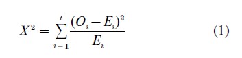
In most practical situations, the values of E₁, E=2, …, E_t involve estimates of the k parameters of the model. Then for large samples , the distribution of X² is approximated by the χ² distribution with t-k-1 degrees of freedom when the probability model is in fact correct (see the discussion in Bishop et al. 1975, for details on conditions associated with the estimates used, etc.). For categorical data problems such as those arising in the analysis of contingency table data, a widely used alternative to X² is the log-likelihood ratio test which is also referred to as the ‘deviance.’ Both of these are members of the power-divergence family of goodnessof-fit statistics proposed by Read and Cressie (1988):

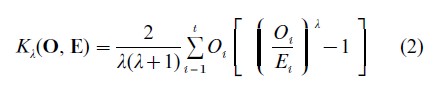
where λ is a real-valued parameter in the interval -∞<λ<∞ . The statistic x² corresponds to λ=1, and the log-likelihood ratio statistic corresponds to the limit as λ→0. All of the members of this power divergence family of statistics are asymptotically equivalent. Read and Cressie (1988) describe some rationales for the choice of value of λ.

To test the fit of a specific model, e.g., the model of independence in a two-way contingency table, the chisquared test uses an omnibus alternative, e.g., dependence. The p-value of the test, is the probability of observing a discrepancy as large or larger than that observed under the hypothesized null distribution, where ‘discrepancy’ is measured by the particular distance metric K_λ(O, E) of equation (2). But in many circumstances testing the goodness of fit of a model is not viewed as being the same as doing a test of hypothesis or test of significance. Not rejecting the null hypothesis at some arbitrary p-value is often taken as evidence that the model provides an acceptable fit to the data (cf. the discussion in Bishop et al. 1975).

Goodness-of-fit test statistics are, of course, sensitive to the sample size n, and to the real class of alternative models of interest. Suppose the null model is not exactly true (as is nearly always the case). Then, with a large enough value of n, one will almost surely conclude that the null model does not fit the data. For modest values of n the situation is more complex, and will result in small p-values for some alternatives, while for others the model may appear to fit the data reasonably well. And if the data are sparse, i.e., if the sample size, n is small relative to the number of cells t, or the number of parameters being estimated k, then the p-value computed by reference to the correspond- ing χ² distribution will inevitably suggest that the model fits even when it does not (cf., Koehler and Larntz 1980). Thus, the p-value of a chi-square test alone gives limited guidance on whether the hypothesized distribution is close enough to being correct that the conclusions of the analysis can be relied upon. When goodness-of-fit tests are used for model comparison and model search some of these problems can be attenuated, as is described in Sect. 3.

2. Other Goodness-Of-fit Approaches Focused On Empirical Distributions

Other classes of goodness-of-fit tests are of special interest when one is focused on the appropriateness of a specific parametric model for some underlying cumulative distribution function, F (x). What is often done in such circumstances is to compute the empirical distribution function F_n(x), whose value at x is the fraction of the sample with values less than or equal to x, i.e., (#x_i≤x) , and then compare F_n(x) with F (x). Well known examples of such tests include the Kolmogorov–Smirnov test, the Cramer–von Mises test, the Anderson–Darling, and the Neyman smooth test. These, and related diagnostics, are described in Goodness-of-fit Tests and Diagnostics.

One of the most widely used diagnostic methods for checking the fit of a model is the quantile–quantile or (Q – Q) plot, which plots the quantiles of the empirical distribution Fn(x), against the quantiles of the assumed distribution F_n(x). A straight line through the origin at a 45 degree slope indicates a perfect fit. The advantage of this method is that it can indicate where in the distribution the assumption is weakest. Q – Q and other probability plots are described in Wilk and Gnanidesikan (1968) and are used in statistical practice. The interpretation of deviations from the line in such plots is, however, often subjective.

3. Classical Approaches To Model Comparison And Model Search

3.1 Model Comparison

Model comparison and model search are ubiquitous activities in modern statistical practice. When analysts consider developing a regression model to describe a set of data, for example, they typically have a large number of possible variables available for inclusion in the model. What is well-known in the regression context is that the use of additional regression variables typically improves the ‘predictive fit’ of the model to the data (e.g., see Copas 1983) but including as many variables as possible is a poor strategy which does not hold up to scrutiny under cross-validation or when predictions are made for new observations (e.g., see the discussion in Copas, 1983, and Linhart and Zucchini 1986). Thus, at a minimum, statistical analysts engage in a series of model comparisons or tests in order to avoid the inclusion of ‘non-significant’ variables or terms in a model. This follows the scientific dictum known as ‘Occam’s razor,’ attributed to William of Occam (but see Thorburn 1918), which suggests that the simpler of two models should be the one chosen. For example, t-tests and F-tests are widely used in model selection procedures for regression and analysis of variance models. Similarly, there are various chi-square test-based techniques for selecting among the class of log linear models applicable for contingency table structures, and these typically (although not always) resemble corresponding model selection procedures for analysis of variance and regression models (see the discussions in Bishop et al. 1975, and Fienberg 1980).

3.2 Model Search

Several methods of penalizing large models to avoid overfitting have been proposed, many taking the form of choosing a model to minimize

where l is the likelihood ratio, f is the penalty assessed for choosing a model with p₁ parameters instead of a more parsimonious one with p₂ parameters, and n is the sample size. When the models are nested, i.e., one is a special case of the other, the quantity -2 log l is the likelihood ratio test for comparing them. Under the null hypothesis that the simpler model fits, this test statistic follows a χ² distribution when the sample size n is sufficiently large.

The choice f ( p₁, p₂, n) =2( p₁– p₂) corresponds to Akaike’s Information Criterion (Akaike 1973) or AIC, while f ( p₁, p₂, n)=( p₁-p₂) log n corresponds to Schwarz’s (1978), also referred to as the Bayesian Information Criterion or BIC. Other classical approaches to this problem include Mallow’s (1973) C_p statistic which is similar to AIC, and Allen’s (1974) PRESS which comes from a related prediction criterion.

These and other related penalized optimization approaches to model selection have been used in the regression setting involving continuous or categorical variables. Edwards (2000), for example, uses both AIC and BIC and suggests variations on computationally efficient model search that take special advantage of the form of graphical models.

4. Bayesian Approaches To Goodness Of Fit

Faced with the question of the adequacy of a particular parametric model, a natural Bayesian impulse is to embed the model in question in a parametric model of higher dimension (see Gelman et al. 1995). Having done so, how should a Bayesian evaluate the special model against the more general alternative?

One answer, espoused especially by George Box (1980) is to use a test of significance. However, the probability of observing an outcome as less or more extreme than that observed is only distantly related to goodness of fit, and violates the likelihood principle.

A second answer, more in keeping with Bayesian ideas, is to impose a prior distribution on the larger parameter space created by embeddings. Every continuous prior distribution in this larger space has the consequence that the original model would have prior, and hence posterior, probability zero. It is for this reason that L. J. Savage advocated models ‘as big as an elephant’ (see Lindley 2000). A second type of prior distribution that might be used takes the form of a spike-and-slab, i.e., one that puts positive probability on the original model (the spike) and a continuous prior on the rest of the space (the slab). The posterior odds on the original model can then be expressed as the product of the prior odds and the ‘Bayes factor.’ Bayes factors have attracted attention because, in the case of only two alternatives, they give a quantity that depends on only the likelihood function and that indicates the strength of the evidence. Faced with more than two alternatives, and especially with a continuum of alternatives, the Bayes factor critically depends on the prior distribution in the alternative space. When the prior is close to the special model, the alternative is favored; when it puts most of its mass far from the special case, the special case is favored, as is reasonable. Attempts to overcome this dependence using heuristics claimed to be robust to changes in the prior on the alternative space include fractional Bayes factors (O’Hagan 1995) and so-called intrinsic Bayes factors (Berger and Perrichi 1996). Another difficulty with Bayes factors, highlighted by Kadane and Dickey (1980) is that the loss function associated with them is two-valued. Hence if the wrong model is chosen, one is assumed not to care whether the error is quantitatively trivial or not. This is an unreasonable way to think about model choice.

Each of these methods is based on the notion that a better model should fit the data better. If this were true, the very best model for any data set would put a probability of one on the data actually observed, so that whatever happened had to have happened. While such a model is useless for prediction, it does show that other considerations such as prior beliefs about how the data might have been generated, and utility considerations, must enter into a full explanation of model choice.

Bayesians too have developed approaches that are analogous to the classical approaches discussed above which penalize large models to avoid ‘overfitting.’ For example, for the problem of variable selection for the normal linear model, George and Foster (2000) provide interpretations of AIC, C_p, BIC, and RIC (for Risk Inflation Criterion) under a specific hierarchical Bayesian formulation. Similarly, Madigan and Raftery (1994) suggest several such strategies using posterior model probabilities, including variations of Occam’s razor in order to discard models with low posterior probability. But there is limited agreement on the theoretical basis for such a strategy. Utility considerations should weigh heavily in choosing the form of a penalized search criteria, and there has not been (and it may not be possible for there to be) a convincing argument as to why a Bayesian’s utility ‘should’ be consistent with one of these forms and not another. By contrast, Leamer (1978) presents a more flexible, but ad hoc Bayesian view of what he terms ‘specification searches.’

Finally, we mention the proposal to use ‘Bayesian model averaging’ (see Hoeting et al. 1999), which combines posterior information across possible models instead of choosing directly from among them. This approach is closely related to some of the efforts to do Bayesian model selection, but has a further difficulty. The interpretation of parameters in a statistical model depends on other parameters in the model. Thus it remains unclear how to interpret posterior distributions for parameters based on combining results across posteriors for different models.

5. Conclusion

Given the goal of assessing whether a hypothesized statistical model or probabilistic distribution is so far from true as to jeopardize the intended use, it would seem wise to inquire as to the intended use. It would also seem wise not to expect a satisfactory procedure to be independent of the intended use. Second, it seems necessary to address the question of jeopardy, i.e., how much of what kind of departures might make invalid the intended inference. Clearly statisticians and others need to devote more effort to this important topic.

Part of the philosophy behind the objective of model search is to do what our recently deceased colleague Herbert Simon (1959) called ‘satisficing,’ that is to find a model that is good enough to capture the main features of the data but which we know is possibly imperfect in various dimensions. The late John Tukey often reminded statisticians and others that ‘the best is the enemy of the good.’ For many data sets and substantive problems, it is often a fruitless task to try to choose the ‘best’ model—one which demonstrably dominates all others and whose assumptions can be shown to be correct. But there may be many ‘good’ models that serve the analyst’s purposes well without one that dominates. It is a good idea to pick one of them. Thus, it seems wise to give up the notion that a model might be ‘true.’ If, instead, models are thought of as useful ways of thinking about the world, choosing a model because of its usefulness is reasonable, even if formal ways of explaining that choice are now lacking.

 Raynor and Best (1989) provide a good technical discussion of specific goodness-of-fit test statistics, and Read and Cressie (1988) give an extended treatment of the power divergence family of statistics and their use for the analysis of categorical data models. Bishop et al. (1975), discuss model search and goodness of fit in the context of categorical data in a form consistent with the philosophical position presented here. Edwards (2000) and Linhart and Zucchini (1986) provide alternative, but useful discussions of related issues for various forms of linear and generalized linear models. Gelman et al. (1995) offer extended advice on Bayesian approaches to model checking.

Bibliography:

1. Akaike H 1973 Information theory and an extension of the maximum likelihood principle. In: Akaike H (ed.) 2nd International Symposium on Information Theory. Akademia Kiado, Budapest, Hungary, pp. 267–81
2. Allen D M 1974 The relationship between variable selection and prediction. Technometrics 16: 125–7
3. Berger O, Pericchi L R 1996 The intrinsic Bayes factor for linear models. In: Bernardo J M, Berger J O, Dawid A P, Smith A F M (eds.) Bayesian Statistics 5. Oxford University Press, Clarendon, Oxford, UK, pp. 25–44
4. Bishop Y M M I, Fienberg S E, Holland P W 1975 Discrete Multivariate Analysis: Theory and Practice. MIT Press, Cambridge, MA
5. Box G 1980 Sampling and Bayes’ inference in scientific modeling and robustness. Journal of the Royal Statistical Society, Series A 143: 383–430
6. Copas J B 1983 Regression, prediction and shrinkage. Journal of the Royal Statistical Society. Series B 45: 311–54
7. Edwards D 2000 Introduction to Graphical Modeling, 2nd edn. Springer-Verlag, New York
8. Fienberg S E 1980 The Analysis of Cross-classified Categorical Data, 2nd edn. MIT Press, Cambridge, MA
9. George E I, Foster D P 2000 Calibration and empirical Bayes variable selection. Biometrika 87: 731–47
10. Gelman A, Carlin J B, Stern H S, Rubin D B 1995 Bayesian Data Analysis. Chapman & Hall, London
11. Hoeting J A, Madigan D, Raftery A E, Volinsky C T 1999 Bayesian model averaging: A tutorial (with discussion). Statistical Science 14: 382–417
12. Kadane Y B, Dickey J O 1980 Bayesian decision theory and the simplification of models. In: Kmenta J, Ramsey J (eds.) Evaluation of Econometric Models. Academic Press, New York, pp. 245–68
13. Koehler K J, Larntz K 1980 An empirical investigation of goodness-of-fit statistics for sparse multinomials. Journal of the American Statistical Association 75: 336–44
14. Leamer E E 1978 Specification Searches: Ad Hoc Inference With Nonexperimental Data. Wiley, New York
15. Lindley D V 2000 The philosophy of statistics (with discussion). The Statistician 49: 293–337 (see p. 307)
16. Linhart H, Zucchini W 1986 Model Selection. Wiley, New York
17. Madigan D, Raftery A E 1994 Model selection and accounting for model uncertainty in graphical models using Occam’s window. Journal of the American Statistical Association 89: 1535–46
18. Mallows C L 1973 Some comments on C_p. Technometrics 15: 661–76
19. O’Hagan A 1995 Fractional Bayes factors for model comparison. Journal of the Royal Statistical Society, Series B 57: 99–138
20. Pearson K 1900 On a criterion that a given system of deviations from the probable in the case of a correlated system of variables is such that it can be reasonably supposed to have arisen from random sampling. Philosophical Magazine, 5th Series 50: 157–75
21. Rayner J C W, Best D J 1989 Smooth Tests of Goodness of Fit. Oxford University Press, Clarendon, Oxford, UK
22. Read T R C, Cressie N A C 1988 Goodness-of-fit Statistics for Discrete Multivariate Data. Springer-Verlag, New York
23. Schwarz G 1978 Estimating the dimension of a model. Annals of Statistics 6: 461–4
24. Simon H A 1959 Theories of decision-making in economics and behavioral science. American Economic Review 49: 253–73
25. Thorburn W M 1918 The myth of Occam’s razor (in Discussion). Mind, New Series 27: 345–53
26. Wilk M B, Gnanadesikan R 1968 Probability plotting methods for the analysis of data. Biometrika 55: 1–17