Monte Carlo Methods And Bayesian Computation Research Paper

Suppose that π(ψ|y, M) ∞ p(ψ| M) f ( y | ψ, M) is the posterior density for a set of parameters ψ ϵ X in a particular Bayesian model M defined by the prior density p(ψ | M) and sampling density or likelihood function f ( y|ψ, M) and that interest centers on the posterior mean η = ∫_R^d ψπ(ψ|y, M ) dψ. As an illustration of this general setting, consider binary data y_i ϵ {0, 1} modeled by the probabilities Pr ( y_i =1|ψ) = Φ(x _iψ), where Φ is the standard normal cumulative distribution function, x_i are covariates and ψ is an unknown vector of parameters. The posterior distribution of ψ given n independent measurement y = ( y₁ ,…, y_n) is proportional to

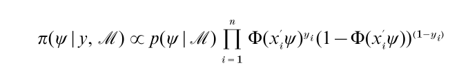
and the goal is to summarize this density.

Now suppose that a sequence of variates {ψ⁽¹⁾,…, ψ^(M)} drawn from π(ψ|y, M ) are available and one computes the sample average of these draws. Under any set of conditions that allow use of the strong law of large numbers, it follows that the sample average is simulation consistent, converging to the posterior mean as the simulation sample M goes to infinity. This then is the essence of the Monte Carlo method: to compute an expectation, or to summarize a given density, sample the density by any method that is appropriate and use the sampled draws to estimate the expectation and to summarize the density.

The sampling of the posterior distribution is, therefore, the central focus of Bayesian computation. One important breakthrough in the use of simulation methods was the realization that the sampled draws need not be independent, that simulation consistency can be achieved with correlated draws. The fact that the sampled variates can be correlated is of immense practical and theoretical importance and is the defining characteristic of Markov chain Monte Carlo methods, popularly referred to by the acronym MCMC, where the sampled draws form a Markov chain. The idea behind these methods is simple and extremely general. In order to sample a given probability distribution, referred to as the target distribution, a suitable Markov chain is constructed with the property that its limiting, invariant distribution is the target distribution. Once the Markov chain has been constructed, a sample of draws from the target distribution is obtained by simulating the Markov chain a large number of times and recording its values. Within the Bayesian framework, where both parameters and data are treated as random variables, and inferences about the parameters are conducted conditioned on the data, the posterior distribution of the parameters provides a natural target for MCMC methods.

Markov chain sampling methods originate with the work of Metropolis et al. (1953) in statistical physics. A crucial and landmark extension of the method was made by Hastings (1970) leading to a method that is now called the Metropolis–Hastings algorithm. This algorithm was first applied to problems in spatial statistics and image analysis (Besag 1974). A resurgence of interest in MCMC methods started with the papers of D. Geman and vs. Geman (1984) who developed an algorithm, a special case of the Metropolis method that later came to be called the Gibbs sampler, to sample a discrete distribution, Tanner and Wong (1987) who proposed a MCMC scheme involving ‘data augmentation’ to sample posterior distributions in missing data problems, and Gelfand and Smith (1990) where the value of the Gibbs sampler was demonstrated for general Bayesian inference with continuous parameter spaces.

2. Marko Chain Monte Carlo Methods

2.1 The Metropolis–Hastings Algorithm

This powerful algorithm provides a general approach for producing a correlated sequence of draws from the target density π(ψ) that may be difficult to sample by a classical independence method. As before, let π(ψ) denote the density that one wishes to sample, where one can assume for simplicity that the density is absolutely continuous; and let q(ψ, ψ´) denote a source density for a candidate draw ψ given the current value ψ in the sampled sequence. The density q(ψ, ψ´) is referred to as the proposal or candidate-generating density. Then, the M–H algorithm is defined by two steps: a first step in which a proposal value is drawn from the candidate-generating density and a second step in which the proposal value is accepted or rejected according to a probability given by

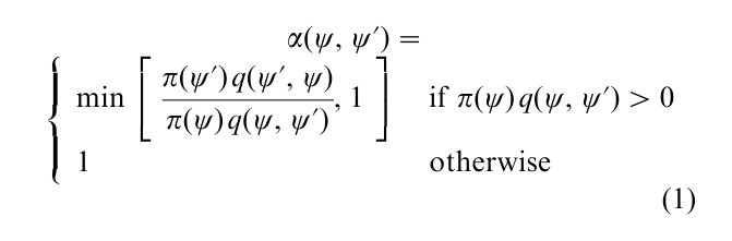
If the proposal value is rejected, then the next sampled value is taken to be the current value; which means that when a rejection occurs the current value is repeated. Given the new value, the same two-step process is repeated and the cycle iterated a large number of times. A full expository discussion of this algorithm, along with a derivation of the method from the logic of reversibility, is provided by Chib and Greenberg (1995).

The M–H method delivers variates from π under quite general conditions. A weak requirement for a law of large numbers for sample averages based on the M–H output involve positivity and continuity of q(ψ, ψ´) for (ψ, ψ´), and connectedness of the support of the target distribution. In addition, if π is bounded then conditions for ergodicity, required to establish the central limit theorem, are satisfied. A discussion of the conditions and the underlying Markov chain theory that justifies these methods was first provided by Tierney (1994) and summarized recently by Robert and Casella (1999). Of course, the variates are from π only in the limit as the number of iterations becomes large but, in practice, after an initial burn-in phase consisting of (say) n iterations, the chain is assumed to have converged and subsequent values are taken as approximate draws from π. Theoretical calculation of the burn-in is not easy, so it is important that the proposal density be chosen to ensure that the chain makes large moves through the support of the target distribution without staying at one place for many iterations. Generally, the empirical behavior of the M–H output is monitored by the autocorrelation time of each component of ψ defined as

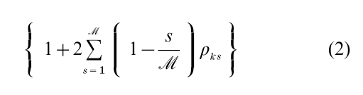
where ρ_ks is the sample autocorrelation at lag s for the kth component of ψ, and by the acceptance rate which is the proportion of times a move is made as the sampling proceeds. Because independence sampling produces an autocorrelation time that is theoretically equal to one, and Markov chain sampling produces autocorrelation times that are bigger than one, it is desirable to tune the M–H algorithm to get values close to one, if possible.

Given the form of the acceptance probability α(ψ, ψ´) it is clear that the M–H algorithm does not require knowledge of the normalizing constant of π(•). Furthermore, if the proposal density satisfies the symmetry condition q(ψ, ψ´) = q(ψ´, ψ), the acceptance probability reduces to π(ψ´) / π(ψ); hence, if π(ψ´) ≥ π(ψ), the chain moves to ψ´, otherwise it moves to ψ with probability given by π(ψ´) / π(ψ). The latter is the algorithm originally proposed by Metropolis et al. (1953).

Different proposal densities give rise to specific versions of the M–H algorithm, each with the correct invariant distribution π. One family of candidate generating densities is given by q (ψ, ψ´) = q(ψ´ – ψ). The candidate ψ´ is thus drawn according to the process ψ´ = ψ + z, where z follows the distribution q, and is referred to as the random walk M–H chain. The random walk M–H chain is perhaps the simplest version of the M–H algorithm and is quite popular in applications. One has to be careful, however, in setting the variance of z because if it is too large it is possible that the chain may remain stuck at a particular value for many iterations while if it is too small the chain will tend to make small moves and move inefficiently through the support of the target distribution.

Hastings (1970) considers a second family of candidate-generating densities that are given by the form q(ψ, ψ´) = q( y). Tierney (1994) refers to this as an independence M–H chain because the candidates are drawn independently of the current location ψ. Chib and Greenberg (1994, 1995) implement such chains by matching the proposal density to the target at the mode by a multivariate normal or multivariate-t distribution with location given by the mode of the target and the dispersion given by inverse of the Hessian evaluated at the mode.

2.2 The Multiple-Block M–H Algorithm

In applications when the dimension of ψ is large it may be preferable, as discussed by Hastings (1970), to construct the Markov chain simulation by first grouping the variables ψ into smaller blocks. For simplicity suppose that two blocks are adequate and that ψ is written as (ψ₁, ψ₂), with ψ_k ϵ Ω_k C R^dk. In that case the M–H algorithm requires the specification of two proposal densities,

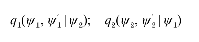
one for each block ψ_k, where the proposal density q_k may depend on the current value of the remaining block. Also, define

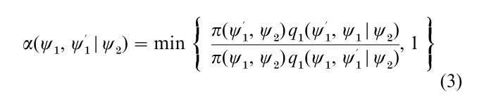
and

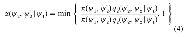
as the probability of move for block ψ_k conditioned on the other block. Then, in what may be called the multiple-block M–H algorithm, one cycle of the algorithm is completed by updating each block, say sequentially in fixed order, using a M–H step with the above probability of move, given the most current value of the other block.

The extension of this method to more than two blocks is straightforward.

2.3 The Gibbs Sampling Algorithm

Another MCMC method, which is a special case of the multiple-block M–H method, is called the Gibbs sampling method and was brought into statistical prominence by Gelfand and Smith (1990). An elementary introduction to Gibbs sampling is provided by Casella and George (1992). To describe this algorithm, suppose that the parameters are grouped into two blocks (ψ₁, ψ₂) and each block is sampled according to the full conditional distribution of block ψ_k, defined as the conditional distribution under π of ψ_k given the other block. In parallel with the multiple-block M–H algorithm, the most current value of the other block is used in deriving the full conditional distribution. Derivation of these full conditional distributions is usually quite simple since, by Bayes’ theorem, each full conditional distribution π (ψ₁| ψ₂) and π (ψ₁|ψ₂ ) are both proportional to π (ψ₁, ψ₂), the joint distribution of the two blocks. In addition, the powerful device of data augmentation, due to Tanner and Wong (1987), in which latent or auxiliary variables are artificially introduced into the sampling, is often used to simplify the derivation and sampling of the full conditional distributions. For further details see Marko Chain Monte Carlo Methods.

3. Implementation Issues

In implementing a MCMC method it is important to assess the performance of the sampling algorithm to determine the rate of mixing and the size of the burnin (both having implications for the number of iterations required to get reliable answers). A large literature has now emerged on these issues, for example Tanner (1996, Sect. 6.3), Cowles and Carlin (1996), Gamerman (1997, Sect. 5.4) and Robert and Casella (1999).

Writing at the turn of the millenium, the more popular approach is to utilize the sampled draws to assess both the performance of the algorithm and its approach to the stationary, invariant distribution. Several such relatively informal methods are now available. Perhaps the simplest and most direct are autocorrelation plots (and autocorrelation times) of the sampled output. Slowly decaying correlations indicate problems with the mixing of the chain. It is also useful in connection with M–H Markov chains to monitor the acceptance rate of the proposal values with low rates implying ‘stickiness’ in the sampled values and thus a slower approach to the invariant distribution.

Somewhat more formal sample-based diagnostics are also available in the literature, as summarized in the routines provided by Best et al. (1995) and now packaged in the BOA program. Although these diagnostics often go under the name ‘convergence diagnostics’ they are in principle approaches that detect lack of convergence. Detection of convergence based entirely on the sampled output, without analysis of the target distribution, is extremely difficult and perhaps impossible. Cowles and Carlin (1996) discuss and evaluate thirteen such diagnostics (for example, those proposed by Geweke (1992), Gelman and Rubin (1992), Zellner and Min (1995), amongst others) without arriving at a consensus.

While implementing MCMC methods it is important to construct samplers that mix well (mixing being measured by the autocorrelation times) because such samplers can be expected to converge more quickly to the invariant distribution. As a general rule, sets of parameters that are highly correlated should be treated as one block when applying the multiple-block M–H algorithm. Otherwise, it would be difficult to develop proposal densities that lead to large moves through the support of the target distribution and the sampled draws would tend to display autocorrelations that decay slowly. Liu (1994) and Liu et al. (1994) discuss possible strategies in the context of three-block Gibbs MCMC chains. Roberts and Sahu (1997) provide further discussion of the role of blocking in the context of Gibbs Markov chains.

4. Additional Uses Of MCMC Methods In Bayesian Inference

MCMC methods provide an elegant solution to the problem of prediction in the Bayesian context. The goal is to summarize the Bayesian predictive density defined as

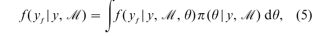
where f ( y_f |y, M , θ) is the conditional density of future observations y_f given ( y, M , θ). In general, the predictive density is not available in closed form. However, this is not a problem when a sample of draws from the posterior density is available. If one simulates

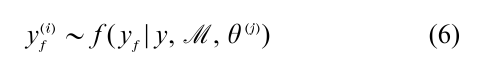
for each sampled draw θ^(j), then the collection of simulated values {y_f⁽¹⁾,…, y_f^{( M)}} is a sample from the Bayes prediction density f (y_f|y, M). The simulated sample can be summarized in the usual way by the computation of sample averages and quantiles.

MCMC methods have also been widely applied to the problem of the model choice. Suppose that there are K possible models M₁,…, M_K for the observed data defined by the sampling densities {f (y|θ_k, M_k)} and proper prior densities { p(θ_k |M_k)} and the objective is to find the evidence in the data for the different models. In the Bayesian approach this question is answered by placing prior probabilities Pr ( M_k) on each of the K models and using the Bayes calculus to find the posterior probabilities {Pr (M₁|y),…, Pr ( M_K|y)} conditioned on the data but marginalized over the unknowns θ_k (Jeffreys 1961 and Kass and Raftery 1995). Specifically, the posterior probability of M_k is given by the expression

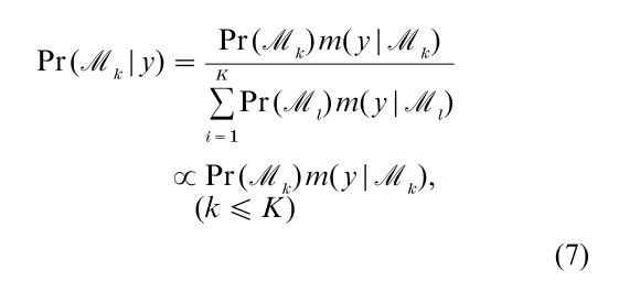
where m( y|M_k) is the marginal likelihood of M_k.

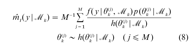
A central problem in estimating the marginal likelihood is that it is an integral of the sampling density over the prior distribution of θ_k. Thus, MCMC methods, which deliver sample values from the posterior density, cannot be used to directly average the sampling density. In addition, taking draws from the prior density to do the averaging produces an estimate that is simulation consistent but highly inefficient because draws from the prior density are not likely to be in high density regions of the sampling density f ( y|θ_k, M_k). A natural way to correct this problem is by the method of importance sampling. If we let h(θ_k |M_k) denote a suitable importance sampling function, then the marginal likelihood can be estimated as

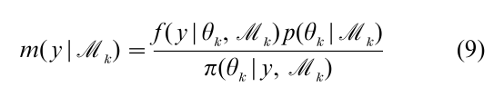
This method is useful when it can be shown that the ratio is bounded, which can be difficult to check in practice, and when the sampling density is not expensive to compute; this, unfortunately, is often not so. Gelfand and Dey (1994) propose an estimator that is based on the posterior simulation output. Another method for finding the marginal likelihood is due to Chib (1995). The marginal likelihood, by virtue of being the normalizing constant of the posterior density, can be expressed as

which is an identity in θ_k. Based on this expression an estimate of the marginal likelihood on the log-scale is given by

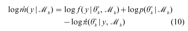
where θ_k* denotes an arbitrarily chosen point and π(θ*_k|y, M_k) is the estimate of the posterior density at that single point. To estimate this posterior ordinate Chib (1995) utilizes the Gibbs output in conjunction with a decomposition of the ordinate into marginal and conditional components. Chib and Jeliazkov (2001) extend that approach for output produced by the Metropolis–Hastings algorithm. A comparison of different estimators of the marginal likelihood is provided by Chen and Shao (1997).

When one is presented with a large collection of candidate models, each with parameters θ_k ϵ B_k C R^dk, direct fitting of each model to find the marginal likelihood can be computationally expensive. In such cases it may be more fruitful to utilize model space– parameter space MCMC algorithms that eschew direct fitting of each model for an alternative simulation of a ‘mega model’ where a model index random variable, denoted as M, taking values on the integers from 1 to K, is sampled in tandem with the parameters. The posterior distribution of M is then computed as the frequency of times each model is visited. Methods for doing this have been proposed by Carlin and Chib (1995) and Green (1995) which are discussed in article 2.1.76. Both methods are closely related as shown by Dellaportas et al. (1998) and Godsill (1998). The problem of variable selection in regression has also been tackled in this context starting with George and McCulloch (1993).

5. An Example

Markov chain Monte Carlo methods have proved enormously popular in Bayesian statistics (see for example, Gilks et al. 1996) where these methods have opened up vistas that were unimaginable fifteen years ago.

As an illustration of how MCMC methods are designed in a Bayesian context, we return to the binary data problem discussed in the introduction and de-scribe the approach of Albert and Chib (1993) that has found many applications. Recall that the posterior distribution of interest is proportional to

where p_i= Φ( x_iψ). To analyze this probit model, and other models for binary and ordinal data, Albert and

Chib introduce latent variables and write z_i = x_iψ + ε_i where ε_i is N (0, 1) and let y_i = I [z_i > 0] where I [•] is the indicator function. This two-equation specification is equivalent to the binary probit regression model since Pr ( y_i=1|ψ) = Pr ( z_i > 0|ψ) = Φ( x_iψ), as required. The Albert–Chib algorithm now consists of simulating the joint posterior distribution of (ψ, Z ), where Z = ( z₁,…, z_n). The MCMC simulation is implemented by sampling the conditional distributions [ψ|y, Z ] and [Z|y, ψ]. The first of these distributions depends only on Z (and not on y) and is obtained by standard Bayesian results on normal linear models. The second factors into a product of independent distributions [z_i|y_i, ψ]. The knowledge of y_i merely restricts the support of the normal distribution z_i|ψ; if y_i = 0, then z_i ≤ 0 and if y_i = 1, then z_i > 0. Suppose that a priori ψ ~ N_k(ψ₀, C₀), where ψ₀ and C₀ are known hyperparameters. Then, a sample of ψ and Z from the posterior distribution is obtained by iterating on the following steps:

(a) sample ψ from the distribution N_k(ψ, C), w here ψ = C(C₀^-1ψ₀ + ∑ⁿ_i=1x_i z_i), C = (B₀^-1 + ∑ⁿ_i=1x_ix_i)^-1;

(b) sample z_i from F N_(-∞,0)(x ψ, 1) if y_i = 0 and from F N_(0,∞) (x_iψ, 1 ) if y_i = 1, where F N_(a,b)( µ, σ²) denotes the N ( µ, σ²) distribution truncated to the region ( a, b).

At this time, considerable work on MCMC methods and applications continues to emerge, a testament to the importance and viability of MCMC methods in Bayesian analysis.

Bibliography:

1. Albert J H, Chib S 1993 Bayesian analysis of binary and polychotomous response data. Journal of the American Statistical Association 88: 669–79
2. Besag J 1974 Spatial interaction and the statistical analysis of lattice systems (with discussion). Journal of the Royal Statistical Society, B Met 36: 192–236
3. Best N G, Cowles M K, Vines S K 1995 CODA: Convergence diagnostics and output analysis software for Gibbs sampling. Technical report, Cambridge MRC Biostatistics Unit
4. Carlin B P, Chib S 1995 Bayesian model choice via Markov chain Monte Carlo methods. Journal of the Royal Statistical Society, B Met 57: 473–84
5. Casella G, George E I 1992 Explaining the Gibbs sampler. American Statistician 46: 167–74
6. Chen M-H, Shao Q-M 1997 On Monte Carlo methods for estimating ratios of normalizing constants. Annals of Statistics 25: 1563–94
7. Chib S 1995 Marginal likelihood from the Gibbs output. Journal of the American Statistical Association 90: 1313–21
8. Chib S, Greenberg E 1994 Bayes inference in regression models with ARMA( p, q) errors. Journal of Econometrics 64: 183– 206
9. Chib S, Greenberg E 1995 Understanding the Metropolis– Hastings algorithm. American Statistician 49: 327–35
10. Chib S, Jeliazkov I 2001 Marginal likelihood from the Metropolis–Hastings output. Journal of the American Statistical Association 96(453): 276–81
11. Cowles M K, Carlin B 1996 Markov Chain Monte Carlo convergence diagnostics: A comparative review. Journal of the American Statistical Association 91: 883–904
12. Dellaportas P, Forster J J, Ntzoufras I 1998 On Bayesian model and variable selection using MCMC. Technical report, University of Economics and Business, Greece
13. Gamerman D 1997 Marko Chain Monte Carlo: Stochastic Simulation for Bayesian Inference. Chapman and Hall, London
14. Gelfand A E, Dey D (1994) Bayesian Model choice: Asymptotics and exact calculations. Journal of the Royal Statistical Society B56: 501–14
15. Gelfand A E, Smith A F M 1990 Sampling-based approaches to calculating marginal densities. Journal of the American Statistical Association 85: 398–409
16. Gelman A, Rubin D B 1992 Inference from iterative simulation using multiple sequence. Statistical Science 4: 457–72
17. Geman D, Geman S 1984 Stochastic relaxation, Gibbs distributions and the Bayesian restoration of images. IEEE Transactions on Pattern Analysis and Machine Intelligence 12: 609–28
18. George E I, McCulloch R E 1993 Variable selection via Gibbs sampling. Journal of the American Statistical Association 88: 881–9
19. Geweke J 1992 Evaluating the accuracy of sampling-based approaches to the calculation of posterior moments. In: Bernardo J M, Berger J O, Dawid A P, Smith A F M (eds.)
20. Bayesian Statistics. New York: Oxford University Press, pp. 169–93
21. Gilks W R, Richardson S, Spiegelhalter D J 1996 Marko Chain Monte Carlo in Practice. Chapman and Hall, London
22. Godsill S J 1998 On the relationship between model uncertainty methods. Technical report, Signal Processing Group, Cambridge University
23. Green P J 1995 Reversible jump Markov chain Monte Carlo computation and Bayesian model determination. Biometrika 82: 711–32
24. Hastings W K 1970 Monte Carlo sampling methods using Markov chains and their applications. Biometrika 57: 97–109
25. Jeffreys H 1961 Theory of Probability, 3rd edn. Oxford University Press, New York
26. Kass R E, Raftery A E 1995 Bayes factors. Journal of the American Statistical Association 90: 773–95
27. Liu J S 1994 The collapsed Gibbs sampler in Bayesian computations with applications to a gene regulation problem. Journal of the American Statistical Association 89: 958–66
28. Liu J S, Wong W H, Kong A 1994 Covariance structure of the Gibbs Sampler with applications to the comparisons of estimators and augmentation schemes. Biometrika 81: 27–40
29. Mengersen K L, Tweedie R L 1996 Rates of convergence of the Hastings and Metropolis algorithms. Annals of Statistics 24: 101–21
30. Metropolis N, Rosenbluth A W, Rosenbluth M N, Teller A H, Teller E 1953 Equations of state calculations by fast computing machines. Journal of Chemical Physics 21: 1087–92
31. Muller P, Erkanli A, West M 1996 Bayesian Curve fitting using multivariate normal mixtures. Biometrika 83: 67–79
32. Robert C P, Casella G 1999 Monte Carlo Statistical Methods. Springer, New York
33. Roberts G O, Sahu S K 1997 Updating schemes, correlation structure, blocking, and parametization for the Gibbs sampler. Journal of the Royal Statistical Society, B Met 59: 291–317
34. Tanner M A 1996 Tools for Statistical Inference,3rd edn. Springer, New York
35. Tanner M A, Wong H W 1987 The calculation of posterior distributions by data augmentation. Journal of the American Statistical Association 82: 528–40
36. Tierney L 1994 Markov chains for exploring posterior distributions (with discussion). Annals of Statistics 22: 1701–62
37. Zellner A, Min C K 1995 Gibbs sampler convergence criteria. Journal of the American Statistical Association 90: 921–7