Time Series Research Paper

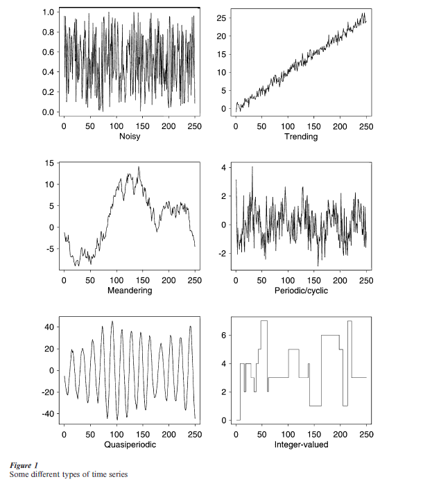
Time series take on a dazzling variety of shapes and forms, indeed there are as many time series as there are functions of real numbers. Some common examples of time series forms are provided in Fig. 1. One notes periods, trends, wandering and integer-values. The time series such as those in the figure may be contemporaneous and a goal may be to understand the interrelationships.

Concepts and fields related to time series include: logitudinal data, growth curves, repeated measures, econometric models, multivariate analysis, signal processing, and systems analysis.

The field, time series analysis, consists of the techniques which when applied to time series lead to improved knowledge. The purposes include summary, decision, description, prediction.

The field has a theoretical side and an applied side. The former is part of the theory of stochastic processes (e.g., representations, prediction, information, limit theorems) while applications often involve extensions of techniques of ‘ordinary’ statistics, for example, regression, analysis of variance, multivariate analysis, sampling. The field is renowned for jargon and acronyms—white noise, cepstrum, ARMA, ARCH (see Granger 1982).

1. Importance

‘… but time and chance happeneth to them all’ (Ecclesiastes).

Time series ideas appear basic to virtually all activities. Time series are used by nature and humans alike for communication, description, and visualization. Because time is a physical concept, parameters and other characteristics is mathematical models for time series can have real-world interpretations. This is of great assistance in the analysis and synthesis of time series.

Time series are basic to scientific investigations. There are: circadian rhythms, seasonal behaviors, trends, changes, and evolving behavior to be studied and understood. Basic questions of scientific concern are formulated in terms of time series concepts— Predicted value? Leading? Lagging? Causal connection? Description? Association? Autocorrelation? Signal? Seasonal effect? New phenomenon? Control? Periodic? Changing? Trending? Hidden period? Cycles?

Because of the tremendous variety of possibilities, substantial simplifications are needed in many time series analyses. These may include assumptions of stationarity, mixing or asymptotic independence, normality, linearity. Luckily such assumptions often appear plausible in practice.

The subject of time series analysis would be important if for no other reason than that it provides means of examining the basic assumption of statistical independence invariably made in ordinary statistics. One of the first commonly used procedures for this problem was the Durbin–Watson test (Durbin and Watson 1950). The autocovariance and spectrum functions, see below, are now often used in this context.

2. History

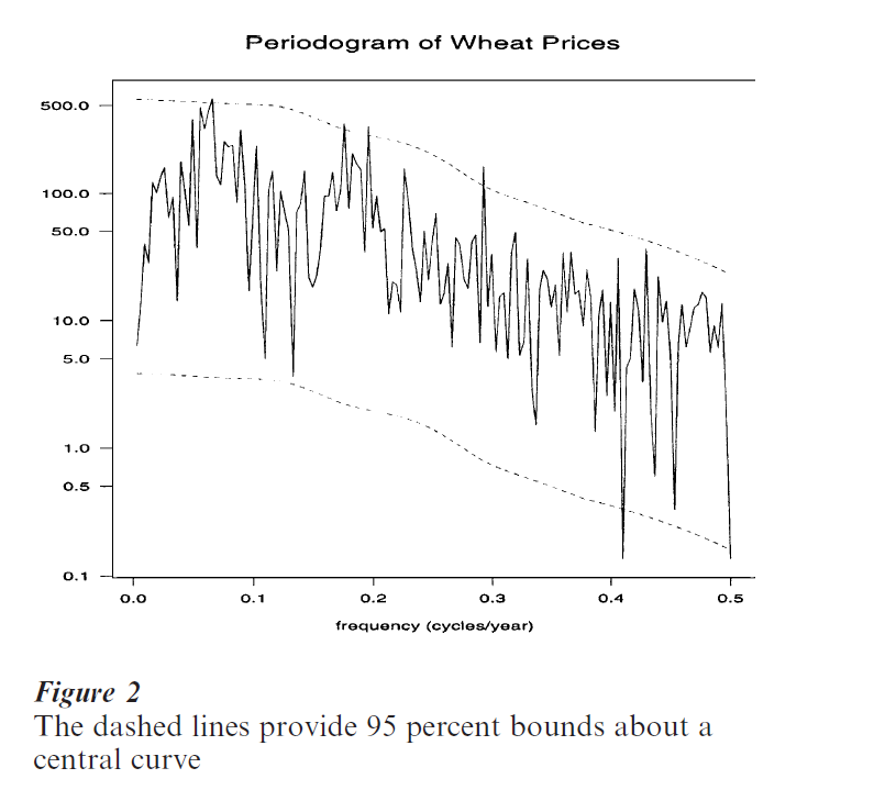
Figure 2 The dashed lines provide 95 percent bounds about a central curve

Contemporary time series analysis has substantial beginnings in both the physical and social sciences. Basic concepts have appeared in each subject and made their way to the other with consequent transfer of technology. Historical researchers important in the development of the field include: Lauritzen (1981), Hooker (1901), Einstein (1914), Wiener (1949), Yule (1927), Fisher (1929), Tukey (1984), Whittle (1951), Bartlett (1966). Books particularly influential in the social sciences include Moore (1914) and Davis (1941). Nowadays many early analyses appear naive. For example, Beveridge in 1920 listed some 19 periods for a wheat price index running from 1500 to 1869 (Beveridge 1922). It is hard to imagine the presence of so much regular behavior in such a series. When statistical uncertainty is estimated using latter-day techniques most of these periods appear insignificant; see the periodogram with 95 percent error bounds in Fig. 2. Many historical references are included in Wold (1965).

Historians of science have made some surprising discoveries concerning early work with time series. An example is presented in Tufte (1983). He shows a time series plot from the tenth or eleventh century AD. This graph is speculated to provide movements of the planets and sun. It is remarkable for its cartesian type character. More generally Tufte remarks, following a study of newspapers and magazines, that ‘The timeseries plot is the most frequently used form of graphic design.’ Casual observation certainly supports Tufte’s study.

Important problems that were addressed in the twentieth century include: seasonal adjustment, leading and lagging indicators, and index numbers. Paradigms that were developed include:

series = signal + noise

series = trend seasonal + noise

series = sum of cosines + noise

series = regression function + noise

These conceptualizations have been used for forecasting, seasonal adjustment and description amongst other things. There are surprises, for example, ordinary least squares is surprisingly efficient in the time series case (see Grenander and Rosenblatt 1957). Other books from the 1950s and 1960s that proved important are Blackman and Tukey (1959), Granger and Hatanaka (1964), Box and Jenkins (1970). Important papers from the era include: Akaike (1965), Hannan (1963) and Parzen (1961).

An important development that began in the 1950s and continues today is the use of recursive computation in the state space model; see Kalman (1963), Harvey (1990), Shumway and Stoffer (2000), and Durbin and Koopman (2001).

3. Basics

3.1 Concepts

There are a number of concepts that recur in time series work. Already defined is the time series, a stretch of values on the same scale indexed by a time parameter. The time parameter may range over the positive and negative integers or all real numbers or subsets of these. Time series data refer to a segment of a time series. A time series is said to have a trend when there is a slowly evolving change. It has a seasonal component when some cyclic movement of period one year is present. (The period of a cyclic phenomenon is the amount of time for it to repeat itself. Its frequency is the reciprocal of the period.)

There is an algebra of mathematical operations that either nature or an analyst may apply to a time series {X(t)} to produce another series {Y(t)}. Foremost is the filter, or linear time invariant operation or system. In the case of discrete equispaced time this may be represented as

t, u = 0, + 1, … An example is the running mean used to smooth a series. The functions X(.), Y(.) may be vector-valued and a(.) may be matrix-valued. In the vector-valued case feedback may be present. The sequence a(u) is called the impulse response function. The operation has the surprising property of taking a series of period P into a series of the same period P. The filter is called realizable when a(u) = 0 for u < 0. Such filters appear in causal systems and when the goal is prediction.

The above ideas concern both deterministic and random series. The latter prove to be important in developing solutions to important problems. Specifically it often proves useful to view the subject of time series as part of the general theory of stochastic processes, that is, indexed families of random variables. One writes {Y(t, ω), t in V}, with ω a random variable and V a set of times. Time series data are then viewed as a segment, {Y(t, ω₀), t = 0,…, T – 1} of the realization labeled by ω , the obtained value of ω. Stochastic time series {Y(t), t = 0, + 1, + 2, …} sometimes are conveniently described by finite dimensional distributions such as

This is particularly the case for time series values with joint normal distributions.

Time series may also be usefully described or generated by stochastic models involving the independent identically distributed random variables of ordinary statistics.

Stochastic models may be distinguished as parametric or nonparametric. Basic parameters of the nonparametric approach include: moments, joint probability and density functions, mean functions, auto-covariance and cross-covariance functions, power spectra.

One basic assumption of time series analysis is that of stationarity. Here the choice of time origin does not affect the statistical properties of the process. For example, the mean level of a stationary series is constant. Basic to time series analysis is handling temporal dependence. To this end one can define the cross-covariance function of the series X and Y at lag u as the covariance of the values X(t + u) and Y(t). In the stationary case this function does not depend on t. In an early paper, Hooker (1901) computed an estimate of this quantity. Another useful parameter is the power spectrum, a display of the intensity or variability of the phenomenon vs. period or frequency. It may be defined as the Fourier transform of the auto-covariance function. The power spectrum proves useful in displaying the serial dependence present, in discovering periodic phenomena and in diagnosing possible models for a series.

In the parametric case there are the autoregressive moving average (ARMA) series. These are regression-type models expressing the value Y(t) as a linear function of a finite number of past values Y(t – 1), Y(t – 2), … of the series and the values ε(t), ε(t – 1), … of a sequence of independent identically distributed random variables. ARMAs have proved particularly useful in problems of forecasting.

Contemporary models for time series are often based upon the idea of state. This may be defined as the smallest entity summarizing the past history of the process. There are two parts to the state space model. First, a state equation that describes how the value of the state evolves in time. This equation may contain a purely random element. Second there is an equation indicating how the available measurements at that time t come from the state value at that time. It too may involve a purely random element. The concept of the state of a system has been basic to physics for many years in classical dynamics and quantum mechanics. The idea was seized upon by control engineers, for example, Kalman (1963) in the late 1950s. The econometricians realized its usefulness in the early 1980s (see Harvey 1990).

A number of specific probability models have been

 studied in depth, including the Gaussian, the ARMA, the bilinear (Granger 1978), various other nonlinear (Tong 1990), long and short memory, ARMAX, ARCH (Einstein 1914), hidden Markov (MacDonald and Zucchini 1997), random walk, stochastic differential equations (Guttorp 1995, Prakasa Rao 1999), and the periodically stationary.

A list of journals where these processes are often discussed is included at the end of this research paper.

3.2 Problems

There are scientific problems and there are associated statistical problems that arise. Methods have been devised for handling many of these. The scientific problems include: smoothing, prediction, association, index numbers, feedback, and control. Specific statistical problems arise directly. Among these are including explanatories in a model, estimation of parameters such as hidden frequencies, uncertainty computation, goodness of fit, and testing.

Special difficulties arise. These include: missing values, censoring, measurement error, irregular sampling, feedback, outliers, shocks, signal-generated noise, trading days, festivals, changing seasonal pattern, aliasing, data observed in two series at different time points.

Particularly important are the problems of association and prediction. The former asks the questions of whether two series are somehow related and what is the strength of any association. Measures of association include: the cross-correlation and the coherence functions. The prediction problem concerns the forecasting of future values. There are useful mathematical formulations of this problem but because of unpredictable human intervention there are situations where guesswork seems just as good.

Theoretical tools employed to address the problems of time series analysis include: mathematical models, asymptotic methods, functional analysis, and transforms.

4. Methods

4.1 Descriptive

Descriptive methods are particularly useful for exploratory and summary purposes. They involve graphs and other displays, simple statistics such as means, medians and percentiles, and the techniques of exploratory data analysis (Tukey 1977).

The most common method of describing a time series is by presenting a graph, see Fig. 1. Such graphs are basic for communication and assessing a situation. There are different types. Cleveland (1985) mentions the connected, symbol, connected-symbol and verticalline displays in particular. Figure 1 presents connected graphs.

Descriptive values derived from time series data include extremes, turning points, level crossings and the periodogram (see Fig. 2 for an example of the latter). Descriptive methods typically involve generating displays using manipulations of time series data via operations such as differencing, smoothing and narrow band filtering.

A display with a long history (Laplace 1825, Wold 1965) is the Buys–Ballot table. Among other things it is useful for studying the presence and character of a phenomenon of period P such as a circadian rhythm. One creates a matrix with entry Y((i – 1)P + j) in row i, column j = 1, …, P and then, for example, one computes column averages. These values provide an estimate of the effect of period P. The graphs of the individual rows may be stacked beneath each other in

 a display. This is useful for discerning slowly evolving behavior.

Descriptive methods may be time-side (as when a running mean is computed), frequency-side (as when a periodogram is computed) or hybrid (as when a sliding window periodogram analysis is employed).

4.2 Parameter Estimation

The way to a solution of many time series problems is via the setting down of a stochastic model. Parameters are constants of unknown values included in the model. They are important because substantial advantages arise when one works within the context of a model. These advantages include: estimated standard errors, efficiency, and communication of results. Often parameter estimates are important because they are fed into later procedures, for example, formulas for forecasting.

General methods of estimating parameters include: method of moments, least squares and maximum likelihood. An important time series case is that of harmonic regression. It was developed in Fisher (1929) and Whittle (1951).

There are parametric and nonparametric approaches to estimation. The parametric has the advantage that if the model is correct, then the estimated coefficients have considerably smaller standard errors.

4.3 Uncertainty Estimation

Estimates without some indication of their uncertainty are not particularly useful in practice. There are a variety of methods used in time series analysis to develop uncertainty measures. If maximum likelihood estimation has been used there are classic (asymptotic) formulas. The delta-method or method of linearization is useful if the quantity of interest can be recognized to be a smooth function of other quantities whose variability can be estimated directly. Methods of splitting the data into segments, such as the jackknife, can have time series variants. A method currently enjoying considerable investigation is the bootstrap (Davison and Hinkley 1997). The assumptions made in validating these methods are typically that the series involved is stationary and mixing.

4.4 Seasonal Adjustment

Seasonal adjustment may be defined as the attempted removal of obscuring unobservable annual components. There are many methods of seasonal adjustment (National Bureau of Economic Research 1976), including state space approaches (Hannan 1963).

The power spectrum provides one means of assessing the effects of various suggested adjustment procedures.

4.5 System Identification

System identification refers to the problem of obtaining a description or model of a system on the basis of a stretch of input to and the corresponding output from a system of interest. The system may be assumed to be linear time invariant as defined above.

In designed experiments the input may be a series of pulses, a sinusoid or white noise. In a natural experiment the input is not under the control of the investigator and this leads to complications in the interpretation of the results. System identification relates to the issue of causality. In some systems one can turn the input off and on and things are clearer.

4.6 Computing

Important computer packages for time series analysis include: Splus, Matlab, Mathematica, SAS, SPSS, TSP, STAMP. Some surprising algorithms have been found: the fast Fourier transform (FFT), fast algorithms from computational geometry, Monte Carlo methods, and the Kalman–Bucy filter. Amazingly a variant of the latter was employed by Thiele in 1880 Lauritzen 1981), while the FFT was known to Gauss in the early 1800s (Heideman et al. 1984).

5. Current Theory And Research

Much of what is being developed in current theory and research is driven by what goes on in practice in time series analyses. What is involved in a time series analysis? The elements include: the question, the experiment, the data, plotting the data, the model, model validation, and model use. The importance of recognizing and assessing the basic assumptions is fundamental.

The approach adopted in practice often depends on how much data are available. In the case that there are a lot of data even procedures that are in some sense inefficient are often used effectively. A change from the past is that contemporary analysis often results from the appearance of very large fine data sets. The amount of data can seem limitless as, for example, in the case of records of computer tasks. There are many hot research topics. One can mention: exploratory data analysis techniques for very large data sets, so-called improved estimates, testing (association? cycle present?), goodness of fit diagnostics. There are the classical and Bayesian approaches, the parametric, semi-parametric, and nonparametric analyses, the problem of dimension estimation and that of reexpression of variables.

Current efforts include research into: bootstrap variants, long-memory processes, long-tailed distributions, nonGaussian processes, unit roots, nonlinearities, better approximations to distributions, demonstrations of efficiency, self-similar processes, scaling relationships, irregularly observed data, doubly stochastic processes as in hidden Markov, cointegration, disaggregation, cyclic stationarity, wavelets, and particularly inference for stochastic differential equations.

Today’s time series data values may be general linear model type (Fahrmein and Tutz 1994), for example, ordinal, state-valued, counts, proportions, angles, ranks. They may be vectors. They may be functions. The time label t may be location in space or even a function. The series may be vector-valued. The data may have been collected in an experimental design.

There are some surprises: the necessity of tapering and prewhitening to reduce bias, the occurrence of aliasing, the high efficiency of ordinary least squares estimates in the correlated case, and the approximate independence of empirical Fourier transform values at different frequencies (Brillinger 1975).

6. Future Directions

It seems clear that time series research will continue on all the existing topics as the assumptions on which any existing problem solution has been based appear inadequate. Further, it can be anticipated that more researchers from nontraditional areas will become interested in the area of time series as they realize that the data they have collected, or will be collecting, are correlated in time.

Researchers can be expected to be even more concerned with the topics of nonlinearity, conditional heteroscedasticity, inverse problems, long memory, long tails, uncertainty estimation, inclusion of explanatories, new analytic models, and properties of the estimates when the model is not true. The motivation for the latter is that time series with unusual structure seem to appear steadily. An example is the data being collected automatically via the World Wide Web. Researchers can be anticipated to be seeking extensions of existing time series methods to processes with more general definitions of the time label— spatial, spatial-temporal, functional, angular. At the same time they will work on processes whose values are more general, even abstract.

More efficient, more robust, and more applicable solutions will be found for existing problems. Techniques will be developed for dealing with special difficulties such as missing data, nonstationarity, outliers. Better approximations to the distributions of time series based statistics will be developed.

Many have stressed the advantages of linear system identification via white noise input. Wiener (1958) stressed the benefits of using Gaussian white noise input. This idea has not been fully developed. Indeed data sets obtained with this input will continually yield to novel analytic methods as they make their appearance.

The principal journals in which newly developed statistical methods for time series are presented and studied include: Journal of Time Series Analysis, Annals of Statistics, Stochastic Processes and their Applications, Journal of the American Statistical Association, Econometrica, IEEE Transactions in Signal Processing.

Bibliography:

1. Akaike H 1965 On the statistical estimation of the frequency response function of a system having multiple input. Annals of the Institute of Statistics and Mathematics 17: 185–210
2. Bartlett M S 1966 Stochastic Processes. Cambridge University Press, Cambridge, UK
3. Beveridge W H 1922 Wheat prices and rainfall in western Europe. Journal of the Royal Statistical Society 85: 412–59
4. Blackman R B, Tukey J W 1959 The Measurement of Power Spectra From the Point of View of Communications Engineering. Dover, New York
5. Box G E P, Jenkins G M 1970 Time Series Analysis: Forecasting and Control. Holden-Day, San Francisco
6. Brillinger D R 1975 Time Series: Data Analysis and Theory. Holt, Rinehart and Winston, New York
7. Cleveland W S 1985 The Elements of Graphing Data. Wadsworth, Belmont, CA
8. Davis H T 1941 The Analysis of Economic Time Series. Principia, Bloomington, IN
9. Davison A C, Hinkley D V 1997 Bootstrap Methods and Their Application. Cambridge University Press, Cambridge, UK
10. Durbin J, Koopman S J 2001 Time Series Analysis by State Space Methods. Oxford University Press, Oxford, UK
11. Durbin J, Watson G S 1950 Testing for serial correlation in least squares regression. Biometrika 37: 409–28
12. Durbin J, Watson G S 1951 Testing for serial correlation in least squares regression. Biometrika 38: 159–77
13. Einstein A 1914 Methode pour la determination des valeurs statistiques d’observations concernant des grandeurs soumises a des fluctuations irregulieres. Archives of Sciences Physiques et Naturelles Series 4 37: 254–5
14. Engle R F (ed.) 1995 ARCH Selected Readings. Oxford University Press, Oxford, UK
15. Fahrmein L, Tutz G 1994 Multivariate Statistical Modelling Based on Generalized Linear Models. Springer, New York
16. Fisher R A 1929 Tests of significance in harmonic analysis. Proceedings of the Royal Society of London A 125: 54–9
17. Granger C W J 1982 Acronyms in time series analysis. Journal of Time Series Analysis 2: 103–8
18. Granger C W J, Andersen A P 1978 An Introduction to Bilinear Time Series Models. Vandenhoeck und Ruprecht, Gottingen
19. Granger C W J, Hatanaka M 1964 Spectral Analysis of Economic Time Series. Princeton University Press, Princeton, NJ
20. Grenander U, Rosenblatt M 1957 Statistical Analysis of Stationary Time Series. Wiley, New York
21. Guttorp P 1995 Stochastic Modelling of Scientific Data. Chapman & Hall, London
22. Hannan E J 1960 Time Series Analysis, Methuen, London
23. Hannan E J 1963 Regression for time series. In: Rosenblatt M (ed.) Time Series Analysis. Wiley, New York
24. Harvey A C 1990 Forecasting, Structural Time Series Models and the Kalman Filter. Cambridge University Press, Cambridge, UK
25. Harvey A C, Koopman S J, Penzer J 1998 Messy time series: A unified approach. Advances in Econometrics 13: 103–43
26. Heideman M T, Jondon D H, Burrus C S 1984 Gauss and the history of the fast Fourier transform. Archives in History and Exact Science 34: 265–77
27. Hooker R H 1901 Correlation of the marriage-rate with trade. Journal of the Royal Statistical Society 64: 696–703
28. Kalman R E 1963 Mathematical description of linear dynamical systems. SIAM Journal of Control 1: 152–92
29. Laplace P S 1825 Traite de Mechanique Celeste. Bachelier, Paris
30. Lauritzen S L 1981 Time series analysis in 1880: A discussion of contributions made by T. N. Thiele. International Statistical Review 49: 319–31
31. MacDonald I L, Zucchini W 1997 Hidden Marko and Other Models for Discretealued Time Series. Chapman and Hall, London
32. Moore H L 1914 Economic Cycles: Their Law and Cause. Macmillan, New York
33. National Bureau of Economic Research Bureau of the Census 1976 Conference on Seasonal Analysis of Economic Time Series. Dept. of Commerce, Bureau of the Census, Washington, DC
34. Parzen E 1961 An approach to time series analysis. Annals of Mathematical Statistics 32: 951–89
35. Prakasa Rao B L S 1999 Statistical Inference for Diffusion Type Processes. Arnold, London
36. Shumway R H, Stoffer D S 2000 Time Series Analysis and its Applications. Springer, New York
37. Tong H 1990 Non-linear Time Series: A Dynamical System Approach. Oxford University Press, New York
38. Tufte E R 1983 The Elements of Graphing Data. Graphics Press, Cheshire, CT
39. Tukey J W 1977 Exploratory Data Analysis. Addision-Wesley, Reading, MA
40. Tukey J W 1984 The Collected Works of John W. Tukey I-II Time Series. Wadsworth, Belmont, CA
41. Whittle P 1951 Hypothesis Testing in Time Series Analysis. Almqvist and Wiksell, Uppsala, Sweden
42. Wiener N 1949 Time Series. MIT Press, Cambridge, MA
43. Wiener N 1958 Nonlinear Problems in Random Theory. MIT Press, Cambridge, MA
44. Wold H O A 1965 Bibliography: on Time Series and Stochastic Processes. MIT Press, Cambridge, MA
45. Yule G U 1927 On the method of investigating periodicities in disturbed series with special reference to Wolfer’s sunspot numbers. Philosophical Transactions A 226: 267–98