Semiparametric Models Research Paper

1. Introduction

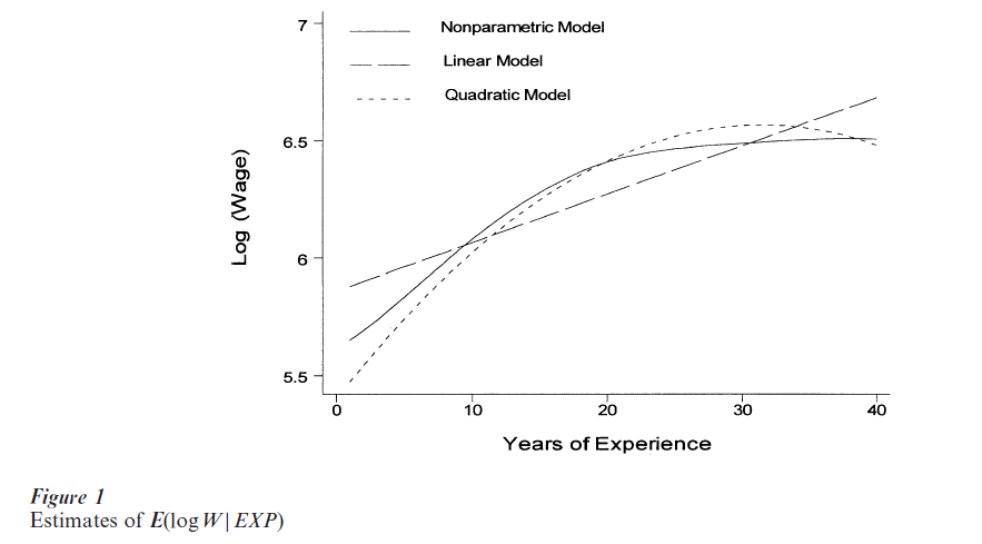
A conditional mean function gives the mean of a dependent variable Y conditional on a vector of explanatory variables X. Denote the mean of Y conditional on X = x by E(Y|x). For example, suppose that Y is a worker’s weekly wage (or, more often in applied econometrics, the logarithm of the wage) and X includes such variables as years of work experience and education, race, and sex. Then E(Y x) is the mean wage (or logarithm of the wage) when experience and the other explanatory variables have the values specified by x. As an illustration, the solid line in Fig. 1 shows an estimate of the mean of the logarithm of weekly wages, log W, conditional on years of work experience, EXP, for white males with 12 years of education who work full time and live in urban areas of the North Central USA. The estimate was obtained by applying a nonparametric method (explained in Sect. 2) to data from the 1993 Current Population Survey (CPS). The estimated conditional mean of log W increases steadily up to approximately 30 years of experience and is flat thereafter.

In most applications, E(Y|x) is unknown and must be estimated from data on the variables of interest. In the case of estimating a wage function, the data consist of observations of individuals’ wages, years of experience, and other characteristics. The most widely used method for estimating E(Y|x) is not the non- parametric method mentioned previously, but rather a method that assumes that E(Y|x) is known up to finitely many constant parameters. This gives a ‘para- metric model’ for E(Y|x). Often, E(Y|x) is assumed to be a linear function of x, in which case the parameters can be estimated by ordinary least squares (OLS), among other ways. A linear function has the form E(Y|x) = β`x, where β is a vector of coefficients. For example, if x consists of an intercept and the two variables x and x , then β has three components, and β`x = β₀ + β₁x₁ + β₂x₂. OLS estimators are described in many textbooks. See, for example, Goldberger (1998).

The OLS estimator of E(Y|x) can be highly misleading if E(Y|x) is not linear in the components of x, that is if there is no β such that E(Y|x) = β`x. This problem is illustrated by the dashed and dotted lines in Fig. 1, which show two parametric estimates of the mean of the logarithm of weekly wages conditional on years of work experience. The dashed line is the OLS estimate that is obtained by assuming that E(log W|EXP) is the linear function E(log W|EXP) = β₀ + β₁ EXP. The dotted line is the OLS estimate that is obtained by assuming that E(log W|EXP) is quadratic: E(log W|EXP) = β₀ + β₁ EXP + β₂ EXP². The nonparametric estimate (solid line) places no restrictions on the shape of E(log W EXP). The linear and quadratic models give misleading estimates of E(log W|EXP). The linear model indicates that E(log W|EXP) steadily increases as experience increases. The quadratic model indicates that E(log W|EXP) decreases after 32 years of experience. In contrast, the nonparametric estimate of E(log W|EXP) becomes nearly flat at approximately 30 years of experience. Because the nonparametric estimate does not restrict the conditional mean function to be linear or quadratic, it is more likely to represent the true conditional mean function.

The opportunities for specification error increase if Y is binary. For example, consider a model of the choice of travel mode for the trip to work. Suppose that the available modes are automobile and transit. Let Y = 1 if an individual chooses automobile and Y= 0 if the individual chooses transit. Let X be a vector of explanatory variables such as the travel times and costs by automobile and transit. Then E(Y|x) is the probability that Y = 1 (the probability that the individual chooses automobile) conditional on X = x. This probability will be denoted P(Y = 1|x). In applications of binary response models, it is often assumed that P(Y|x) = G(β`x), where β is a vector of constant coefficients and G is a known probability distribution function. Often, G is assumed to be the cumulative standard normal distribution function, which yields a ‘binary probit’ model, or the cumulative logistic distribution function, which yields a ‘binary logit’ model. The coefficients β can then be estimated by the method of maximum likelihood (Amemiya 1985). However, there are now two potential sources of specification error. First, the dependence of Y on x may not be through the linear index β`x. Second, even if the index β`x is correct, the ‘response function’ G may not be the normal or logistic distribution function. See Horowitz (1993, 1998) for examples of specification errors in binary response models and their consequences.

Many investigators attempt to minimize the risk of specification error by carrying out a ‘specification search’ in which several different models are estimated and conclusions are based on the one that appears to fit the data best. Specification searches may be unavoidable in some applications, but they have many undesirable properties and their use should be minimized. There is no guarantee that a specification search will include the correct model or a good approximation to it. If the search includes the correct model, there is no guarantee that it will be selected by the investigator’s model selection criteria. Moreover, the search process invalidates the statistical theory on which inference is based.

The rest of this entry describes methods that deal with the problem of specification error by relaxing the assumptions about functional form that are made by parametric models. The possibility of specification error can be essentially eliminated through the use of nonparametric estimation methods. These are described in Sect. 2. They assume that E(Y|x) is a smooth function but make no other assumptions about its shape or functional form. However, nonparametric methods have important disadvantages that seriously limit their usefulness in applications. Semiparametric methods, which are described in Sect. 3 offer a compromise. They make assumptions about functional form that are stronger than those of a nonparametric model but less restrictive than the assumptions of a parametric model, thereby reducing (though not eliminating) the possibility of specification error. In addition semiparametric methods avoid the most serious practical disadvantages of nonparametric methods.

2. Nonparametric Models

In nonparametric estimation E(Y|x) is assumed to satisfy smoothness conditions such as differentiability, but no assumptions are made about its shape or the form of its dependence on x. Hardle (1990) and Fan and Gijbels (1996) provide detailed discussions of nonparametric estimation methods. One easily understood and frequently used method is called ‘kernel estimation.’ This method was used to produce the solid line in Fig. 1. To describe the kernel method simply, assume that X is a continuously distributed, scalar random variable. Let {Y_i, X_i : i =1, …, n } be a random sample of n observations of (Y, X ). Let K be a probability density function that is bounded, continuous, and symmetrical about zero. For example, K may be the standard normal density function. Let {h_n} to be a sequence of positive numbers that converges to 0 as n → ∞. For each n = 1, 2, … and i = 1, …, n define the function w_ni( ) by

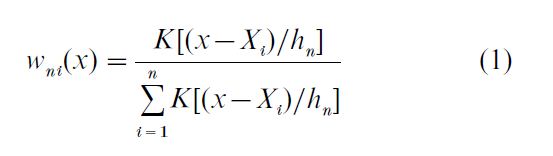
Then the kernel nonparametric estimator of E(Y|x) is

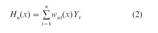
H_n(x) is a weighted average of the observed values of Y. Observations Y_i for which X_i is close to x get higher weight than do observations for which X_i is far from x. It can be shown that if h_n → 0 and nh_n / (log n) → ∞ as n → ∞, then H_n(x) → E(Y|x) with probability 1. Thus, if n is large, H_n(x) is likely to be very close to E(Y|x). Hardle (1990) provides a detailed discussion of the statistical properties of kernel nonparametric estimators.

Nonparametric estimation minimizes the risk of specification error, but the price of this flexibility can be high. One important reason for this is that the precision of a nonparametric estimator decreases rapidly as the number of continuously distributed components of X increases. This phenomenon is called the ‘curse of dimensionality.’ As a result of it, impracticably large samples are usually needed to obtain acceptable estimation precision if X is multidimensional, as it often is in social science applications. For example, a labor economist may want to estimate mean log wages conditional on years of work experience, years of education, and one or more indicators of skill levels, thus making the dimension of X at least 3. See Exploratory Data Analysis: Multi ariate Approaches (Nonparametric Regression) for further discussion of the curse of dimensionality.

Another problem is that nonparametric estimates can be difficult to display, communicate, and interpret when X is multidimensional. Nonparametric estimates do not have simple analytic forms, so displaying and interpreting them can be difficult. If X is one-or two-dimensional, then the estimate of E(Y|x) can be displayed graphically as in Fig. 1, but only reduceddimension projections can be displayed when X has three or more components. Many such displays and much skill in interpreting them can be needed to fully convey and comprehend the shape of the estimate of E(Y|x).

Another problem with nonparametric estimation is that it does not permit extrapolation. That is, it does not provide predictions of E(Y|x) at points x that are outside of the support (or range) of the random variable X. This is a serious drawback in policy analysis and forecasting, where it is often important to predict what might happen under conditions that do not exist in the available data. Finally, in nonparametric estimation, it can be difficult to impose restrictions suggested by economic or other theory. Matzkin (1994) discusses this issue.

Semiparametric methods permit greater estimation precision than do nonparametric methods when X is multidimensional. In addition, semiparametric estimates are easier to display and interpret than non- parametric ones and provide limited capabilities for extrapolation and imposing restrictions derived from economic or other theory models.

3. Semiparametric Models

The term ‘semiparametric’ refers to models in which there is an unknown function in addition to an unknown finite dimensional parameter. For example, the binary response model P(Y = 1|x) = G( β`x) is semiparametric if the function G and the vector of coefficients β are both treated as unknown quantities. This section describes two semiparametric models of conditional mean functions that are important in applications. The section also describes a related class of models that have no unknown finite-dimensional parameters but, like semiparametric models, mitigate the disadvantages of fully nonparametric models.

In addition to the estimation of conditional mean functions, semiparametric methods can be used to estimate conditional quantile and hazard functions, binary response models in which there is heteroskedasticity of unknown form, transformation models, and censored and truncated mean and medianregression models, among others. Space does not permit discussion of these models here. Horowitz (1998) and Powell (1994) provide more comprehensive treatments in which these models are discussed.

3.1 Single Index Models

In a semiparametric single index model, the conditional mean function has the form

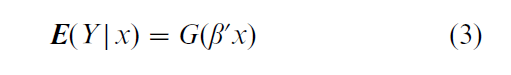
where β is an unknown constant vector and G is an unknown function. The quantity β`x is called an ‘index.’ The inferential problem is to estimate G and β from observations of (Y, X). G in (3.1) is analogous to a link function in a generalized linear model, except in Eqn. (3) G is unknown and must be estimated.

Model (3) contains many widely used parametric models as special cases. For example, if G is the identity function, then Eqn. (3) is a linear model. If G is the cumulative normal or logistic distribution function, then Eqn. (3) is a binary probit or logit model. When G is unknown, Eqn. (3) provides a specification that is more flexible than a parametric model but retains many of the desirable features of parametric models, as will now be explained.

One important property of single index models is that they avoid the curse of dimensionality. This is because the index β`x aggregates the dimensions of x, thereby achieving ‘dimension reduction.’ Consequently, the difference between the estimator of G and the true function can be made to converge to zero at the same rate that would be achieved if β`x were observable. Moreover, β can be estimated with the same rate of convergence that is achieved in a parametric model. Thus, in terms of the rates of convergence of estimators, a single index model is as accurate as a parametric model for estimating β and as accurate as a one-dimensional nonparametric model for estimating G. This dimension reduction feature of single index models gives them a considerable advantage over nonparametric methods in applications where X is multidimensional and the single index structure is plausible.

A single-index model permits limited extrapolation. Specifically, it yields predictions of E(Y|x) at values of x that are not in the support of X but are in the support of β`X. Of course, there is a price that must be paid for the ability to extrapolate. A single index model makes assumptions that are stronger than those of a nonparametric model. These assumptions are testable on the support of X but not outside of it. Thus, extrapolation (unavoidably) relies on untestable assumptions about the behavior of E(Y|x) beyond the support of X.

Before β and G can be estimated, restrictions must be imposed that insure their identification. That is, β and G must be uniquely determined by the population distribution of (Y, X ). Identification of single index models has been investigated by Ichimura (1993) and, for the special case of binary response models, Manski (1988). It is clear that β is not identified if G is a constant function or there is an exact linear relation among the components of X (perfect multicollinearity). In addition, (3.1) is observationally equivalent to the model E(Y|X ) = G*(γ + δβ`x), where γ and δ ≠ 0 are arbitrary and G* is defined by the relation G*(γ + δν) = G(ν) for all ν in the support of β`X. Therefore, β and G are not identified unless restrictions are imposed that uniquely specify γ and δ. The restriction on γ is called ‘location normalization’ and can be imposed by requiring X to contain no constant (intercept) component. The restriction on δ is called ‘scale normalization.’ Scale normalization can be achieved by setting the β coefficient of one component of X equal to one. A further identification requirement is that X must include at least one continuously distributed component whose β coefficient is nonzero. Horowitz (1998) gives an example that illustrates the need for this requirement. Other more technical identification requirements are discussed by Ichimura (1993) and Manski (1988).

The main estimation challenge in single index models is estimating β. Given an estimator b_n of β, G can be estimated by carrying out the nonparametric regression of Y on b_n `X (e.g., by using the kernel method described in Sect. 2). Several estimators of β are available. Ichimura (1993) describes a nonlinear least squares estimator. Klein and Spady (1993) describe a semiparametric maximum likelihood estimator for the case in which Y is binary. These estimators are difficult to compute because they require solving complicated nonlinear optimization problems. Powell et al. (1989) describe a ‘densityweighted average derivative estimator’ (DWADE) that is noniterative and easily computed. The DWADE applies when all components of X are continuous random variables. It is based on the relation

where p is the probability density function of X and the second equality follows from integrating the first by parts. Thus, β can be estimated up to scale by estimating the expression on the right-hand side of the second equality. Powell et al. (1989) show that this can be done by replacing p with a nonparametric estimator and replacing the population expectation E with a sample average. Horowitz and Hardle (1996) extend this method to models in which some components of X are discrete. They also give an empirical example that illustrates the usefulness of single index models. Ichimura and Lee (1991) investigate a multiple index generalization of Eqn. (3).

3.2 Partially Linear Models

In a partially linear model, X is partitioned into two nonoverlapping subvectors, X₁ and X₂. The model has the form

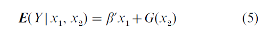
where β is an unknown constant vector and G is an unknown function. This model is distinct from the class of single index models. A single index model is not partially linear unless G is a linear function. Conversely, a partially linear model is a single index model only in this case. Stock (1989, 1991) and Engle et al. (1986) illustrate the use of Eqn. (5) in applications. Identification of β requires the ‘exclusion restriction’ that none of the components of X1 are perfectly predictable by components of X₂. When β is identified, it can be estimated with an n^-1/2 rate of convergence regardless of the dimensions of X and X . Thus, the curse of dimensionality is avoided in estimating β.

An estimator of β can be obtained by observing that Eqn. (5) implies

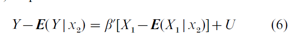
where U is an unobserved random variable satisfying E(U|x₁ , x₂) = 0. Robinson (1988) shows that under regularity conditions β can be estimated by applying OLS to Eqn. (6) after replacing E(Y|x₂) and E(X₁ |x₂) with nonparametric estimators. The estimator of β, b_n, converges at rate n ^-1/2 and is asymptotically normally distributed. G can be estimated by carrying out the nonparametric regression of Y -b _nX₁ on X₂ . Unlike b_n, the estimator of G suffers from the curse of dimensionality; its rate of convergence decreases as the dimension of X₂ increases.

3.3 Nonparametric Additive Models

Let X have d continuously distributed components that are denoted X₁,… X_d. In a nonparametric additive model of the conditional mean function,

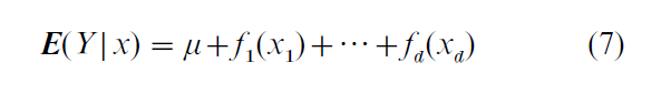
where µ is a constant and f₁, …, f_d are unknown functions that satisfy a location normalization condition such as

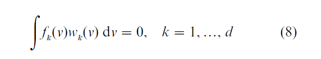
where w_k is a non-negative weight function. An additive model is distinct from a single index model unless E(Y|x) is a linear function of x. Additive and partially linear models are distinct unless E(Y|x) is partially linear and G in Eqn. (5) is additive.

An estimator of f_k(k = 1, …, d ) can be obtained by observing that Eqn. (7) and (8) imply

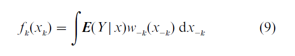
where x_−k is the vector consisting of all components of x except the kth and w_−k is a weight function that satisfies ∫w_−k(x_−k) dx_−k = 1. The estimator of f_k is obtained by replacing E(Y|x) on the right-hand side of Eqn. (9) with nonparametric estimators. Linton and Nielsen (1995) and Linton (1997) present the details of the procedure and extensions of it. Under suitable conditions, the estimator of f_k converges to the true f_k at rate n^-2/5 regardless of the dimension of X. Thus, the additive model provides dimension reduction. It also permits extrapolation of E(Y|x) within the rectangle formed by the supports of the individual components of X. Hastie and Tibshirani (1990) and Exploratory Data Analysis: Multivariate Approaches (Nonparametric Regression) discuss an alternative estimation procedure called ‘backfitting.’ This procedure is widely used, but its asymptotic properties are not yet well understood.

Linton and Hardle (1996) describe a generalized additive model whose form is

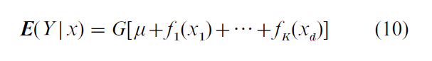
where f₁, …, f_d are unknown functions and G is a known, strictly increasing (or decreasing) function. Horowitz (2001) describes a version of Eqn. (10) in which G is unknown. Both forms of Eqn. (10) achieve dimension reduction. When G is unknown, Eqn. (10) nests additive and single index models and, under certain conditions, partially linear models.

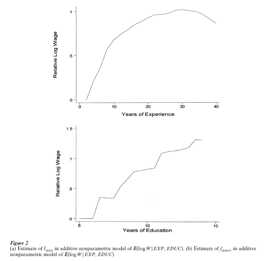
The use of the nonparametric additive specification (7) can be illustrated by estimating the model

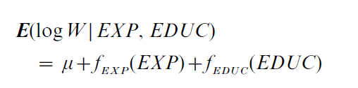
where W and EXP are defined as in Sect. 1, and EDUC denotes years of education. The data are taken from the 1993 CPS and are for white males with 14 or fewer years of education who work full time and live in urban areas of the North Central US. The results are shown in Fig. 2. The unknown functions f_EXP and f_EDUC are estimated by the method of Linton and Nielsen (1995) and are normalized so that f_EXP(2) = f_EDUC(5) = 0. The estimates of f_EXP (Fig. 2a) and f_EDUC (Fig. 2b) are nonlinear and differently shaped. Functions f_EXP and f_EDUC with different shapes cannot be produced by a single index model, and a lengthy specification search might be needed to find a parametric model that produces the shapes shown in Fig. 2. Some of the fluctuations of the estimates of f_EXP and f_EDUC may be artifacts of random sampling error rather than features of E(log W|EXP, EDUC). However, a more elaborate analysis that takes account of the effects of random sampling error rejects the hypothesis that either function is linear.

4. Conclusions

This research paper has described several semiparametric methods for estimating conditional mean functions. These methods relax the restrictive assumptions made by linear and other parametric models, thereby reducing (though not eliminating) the likelihood of seriously misleading inference. The value of semiparametric methods in empirical research has been demonstrated. Their use is likely to increase as their availability in commercial statistical software packages increases.

Bibliography:

1. Amemiya T 1985 Advanced Econometrics. Harvard University Press, Cambridge, MA
2. Engle R F, Granger C W J, Rice J, Weiss A 1986 Semiparametric estimates of the relationship between weather and electricity sales. Journal of the American Statistical Association 81: 310–20
3. Fan J, Gijbels I 1996 Local Polynomial Modelling and its Applications. Chapman & Hall, London
4. Goldberger A S 1998 Introductory Econometrics. Harvard University Press, Cambridge, MA
5. Hardle W 1990 Applied Nonparametric Regression. Cambridge University Press, Cambridge, UK
6. Hastie T J, Tibshirani R J 1990 Generalized Additi e Models. Chapman & Hall, London
7. Horowitz J L 1993 Semiparametric and nonparametric estimation of quantal response models. In: Maddala G S, Rao C R, Vinod H D (eds.) Handbook of Statistics. Elsevier, Amsterdam, Vol. II, pp. 45–72
8. Horowitz J L 1998 Semiparametric Methods in Econometrics. Springer-Verlag, New York
9. Horowitz J L 2001 Nonparametric estimation of a generalized additive model with an unknown link function. Econometrica 69: 599–631
10. Horowitz J L, Hardle W 1996 Direct semiparametric estimation of single-index models with discrete covariates. Journal of the American Statistical Association 91: 1632–40
11. Ichimura H 1993 Semiparametric least squares (SLS) and weighted SLS estimation of single-index models. Journal of Econometrics 58: 71–120
12. Ichimura H, Lee L-F 1991 Semiparametric least squares estimation of multiple index models: single equation estimation. In: Barnett W A, Powell J, Tauchen G (eds.) Nonparametric and Semiparametric Methods in Econometrics and Statistics. Cambridge University Press, Cambridge, UK, pp. 3–49
13. Klein R W, Spady R H 1993 An efficient semiparametric estimator for binary response models. Econometrica 61: 387–421
14. Linton O B 1997 Efficient estimation of additive nonparametric regression models. Biometrika 84: 469–73
15. Linton O B, Hardle W 1996 Estimating additive regression models with known links. Biometrika 83: 529–40
16. Linton O B, Nielsen J P 1995 A kernel method of estimating structured nonparametric regression based on marginal integration. Biometrika 82: 93–100
17. Manski C F 1988 Identification of binary response models. Journal of the American Statistical Association 83: 729–38
18. Matzkin R L 1994 Restrictions of economic theory in nonparametric methods. In: Engle R F, McFadden D L (eds.) Handbook of Econometrics. North-Holland, Amsterdam, Vol. 4, pp. 2523–58
19. Powell J L 1994 Estimation of semiparametric models. In: Engle R F, McFadden D L (eds.) Handbook of Econometrics. NorthHolland, Amsterdam, Vol. 4, pp. 2444–521
20. Powell J L, Stock J H, Stoker T M 1989 Semiparametric estimation of index coeffi Econometrica 51: 1403–30
21. Robinson, P M 1988 Root-N-consistent semiparametric regression. Econometrica 56: 931–54
22. Stock J H 1989 Nonparametric policy analysis. Journal of the American Statistical Association 84: 567–75
23. Stock J H 1991 Nonparametric policy analysis: An application to estimating hazardous waste cleanup benefits. In: Barnett W A, Powell J, Tauchen G (eds.) Nonparametric and Semiparametric Methods in Econometrics and Statistics. Cambridge University Press, Cambridge, UK, pp. 77–98