Distribution Of Simultaneous Equation Estimates Research Paper

These variables are measures of the level of economic activity of a nation. In the production function, Y increases if the inputs K and/or L increase. C increases if Y increases in the consumption equation. Each equation is modeled to explain the variation in the left-hand side ‘explained’ variable by the variation in the right-hand side ‘explanatory’ variables. Error terms are added to analyze numerically the effect of the neglected factors from the right-hand side of the equation. These equations are different from the regression equations since the ‘explained’ variable Y is the ‘explanatory’ variable in the C equation, and Y and C are simultaneously determined by the two equations. Estimation of unknown coefficients and the properties of estimation methods are not straightforward compared with the ordinary least squares estimator.

In practice, this kind of simultaneous equation system is extended to include more than 100 equations, and regularly updated to measure the economic activities of a nation. It is indispensable to analyze numerically the effect of policy changes and public investments.

In this research paper, the statistical model and the estimation methods of all the equations are first explained, followed by the estimation methods of a single equation and their asymptotic distributions. Explained next are the exact distributions, the asymptotic expansions, and the higher order efficiency of the estimators.

1. The System Of Simultaneous Equations And Identification Of The System

We write the structural form of a system consisting of G simultaneous equations as

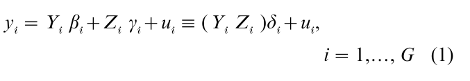
where y_i and Y_i are 1 and G_i subcolumns in the T × G matrix of whole endogenous variables Y = ( y_i, Y_i, Y_ei), Z_i consists of K_i subcolumns in the T × K matrix of whole exogenous variables Z, β_i and γ_i are G_i × 1 and K_i × 1 column vectors of unknown coefficients, δ_i = ( β_i , γ_i´)´, and u_i is the T × 1 error term. This system of G equations with T observations is frequently summarized in a simple form

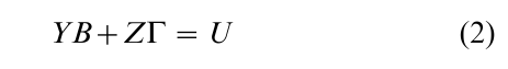
the ith column of which is y_i – Y_iβi – Z_iγi = u_i, i.e., Eqn. (1). The ith columns of B and Γ may be denoted as b_i and c_i where (G – G_i – 1) and (K – K_i) elements are zero so that y_i – Y_iβi – Z_iγi – Y_bi – Z_ci. Zero elements are called zero restrictions. It is assumed that each row of U is independently distributed as N(0, Σ). The reduced form of Eqn. (2) is

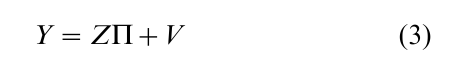
where the K × G reduced form coefficient matrix is Π = -ΓB⁻¹, and the T × G reduced form error term is V = UB⁻¹. Each row of V is assumed to be independently distributed as N(0, Ω), and then Σ = B⁻¹, ΩB⁻¹.

The definition Π = -ΓB⁻¹, or -ΠB = Γ is the key to identify structural coefficients. Coefficients in β_i are identified if they can be uniquely determined by the equation -Π b_i = c_i given Π. This equation is reduced to -Π₀(1, β_i´) = 0 denoting the (K – K_i) × (1 + G_i) submatrix in Π as Π₀. (Rows and columns are selected according to the zero elements in ci and non-zero elements in bi, respectively.) Given Π₀, this includes (K – K_i) linear equations and G_i unknowns, and β_i is solvable if rank (Π₀) = G_i. This means (K – K_i) must be at least G_i, or L = K – K_i – G_i must be at least 0. If L = 0, β_i is uniquely determined. For the positive L, there are L linearly dependent rows in Π₀ since only G_i rows are necessary to determine β_i uniquely. Once β_i is determined, γ_i is determined by other K_i equations through -Πb_i = c_i. L is called the number of the degrees of overidentifiability of the ith equation. Structural coefficients are not uniquely estimable if they are not identified.

2. Estimation Methods Of The Whole System And The Asymptotic Distribution

The full information maximum likelihood (FIML) estimator of all nonzero structural coefficients δ_i, i = 1,…, G, follows from Eqn. (3). Since it is in a linear regression form, the likelihood function can first be minimized with respect to Ω. Once Ω is replaced by the first-order condition, the likelihood function is concentrated where only B and Γ are unknown. The concentrated likelihood function is proportional to

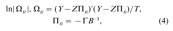
and all zero restrictions are included in B and Γ matrices. In the FIML estimation, it is necessary to minimize |Ω_R| with respect to all non-zero structural coefficients.

The FIML estimator is consistent, and the asymptotic distribution is derived by the central limit theorem. Stacking δ_i, i = 1,…, G in a column vector δ, the FIML estimator δ asymptotically approaches N(0, -I^-1) as follows:

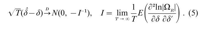
I is the limit of the average of the information matrix, i.e., I⁻¹ is the asymptotic Cramer–Rao lower bound. Then the FIML estimator is the best among consistent and asymptotically normal (BCAN) estimators.

The right-hand side endogenous variable Y_i in (1) is defined by a set of G_i columns in (3) such as Y_i = ZΠ_i + V_i. By the definition of V, Y_i or, equivalently, V_i is correlated with u_i since columns in U are correlated with each other. The least squares estimator applied to (1) is inconsistent because of the correlation between Y_i and u_i. Since Z is assumed to be not correlated with U in the limit, Z is used as K instruments in the instrumental variable method estimator. Premultiplying Z´ to (1), it follows that

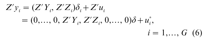
where the K × 1 transformed right-hand side variables Z´Y_i is not correlated with u* in the limit. Stacking all G transformed equations in a column form, the G equations are summarized as w = Xδ +u* where w and u* stack Z´y_i and u*_i, i = 1,…, G, respectively, and are GK × 1. The covariance between u_i* and u_j* is σ_ij(Z´Z) which is the ith row and jth column sub-block in the covariance matrix of u*. (The whole covariance matrix can be written as Σ©(Z´Z) where © signifies the Kroneker product.) Once Σ is estimated consistently (by the 2SLS method explained in the next section), δ is efficiently estimated by the generalized least squares method

This is the three-stage least squares (3SLS) estimator by Zellner and Theil (1962). The assumption of the normal distribution error is not required in this estimation. The 3SLS estimator is consistent and is BCAN since it has the same asymptotic distribution as the FIML estimator.

3. Estimation Methods Of A Single Equation And The Asymptotic Distribution

An alternative way of estimating structural coefficients is to pick up one structural equation, the ith, in a Gequation system, and estimate δ_i neglecting zero restrictions in other equations. Because of this, the other (G – 1) structural equations can be rewritten equivalently as (G – 1) reduced form equations. The limited information maximum likelihood (LIML) estimator by Anderson and Rubin (1949) applies the FIML method to a (1 + G_i)-equation system consisting of (1) and Y_i = ZΠ_i+ V_i. This means the first column and the second G_i columns of B are (1, -β_i´)´ and (0, I )´, respectively, and the first column and the second G_i columns of Γ are (γ_i´, 0´)´ and Π_i, respectively. (If we denote Y as (y_i,Y_i,Y_ei), Y_ei is weakly exogenous in estimating (1) or, equivalently, the structural and reduced form parameters of ( y_i, Y_i) given Y_ei are variation-free from the reduced form coefficient of Y_ei. Then Y_ei is omitted from (2), (3), (4), and (8).) Using these limited information B and Γ matrices, we minimize |Ω_R| with respect to δ_i and Π_i. Defining P_F = F(F´F)⁻¹ F for any full column matrix F, G = (y_i, Y_i)´(P_Z – P_Zi)(y_i, Y_i), and C = (y_i, Y_i)´(I – P_Z)(y_i, Y_i), it turns out that β_i is estimated by minimizing the least variance ratio

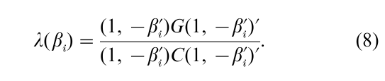
γ_i is estimated by the least squares method applied to (1) replacing β_i with the estimator.

The two stage least squares (2SLS) estimator is the generalized least squares estimator applied to Eqn. (6) using Z´Z as the weight matrix. (See Eqn. (10), where k is set to 1.) The assumption of the normal distribution of the error term is not required in this estimation. Both LIML and 2SLS estimators are consistent, and the large sample distribution is

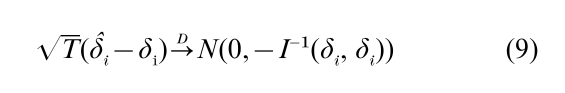
where I is calculated similarly to Eqn. (5) but Ω_R is defined using the limited information B and Γ matrices, and only the diagonal submatrix of I^-1 which corresponds to δ_i is used. (Partial derivatives are calculated with respect to δ_i and columns in Π_i.) This asymptotic distribution is a particular case of Eqn. (5). Both estimators are consistent and BCAN under the zero restrictions imposed on Eqn. (1).

The k-class estimator δ_i(k) unifies both LIML and 2SLS estimators (Theil 1961). It is

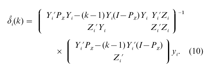
This is the least squares estimator, the 2SLS estimator, and the LIML estimator when k is 0, 1, and 1 + λ, respectively. There are two important properties in the k-class estimator. It is consistent if p lim _{T → ∞} k = 1, and is BCAN if p lim _{T → ∞} √T(k – 1) = 0. If k satisfies these conditions, the k-class estimator is consistent and BCAN even when Y_i´(I – P_Z)Y_i and Y_i´(I – P_Z)y_i are replaced with any matrix and a vector of order O_P(T´).

4. Exact Distributions Of The Single-Equation Estimators

Several early studies compared the bias and mean squared errors of OLS, LIML, 2SLS, FIML, and 3SLS estimators by the Monte Carlo simulations since all but OLS estimators are consistent and are indistinguishable. The OLS estimator was often found as reliable as other consistent estimators. Later, the studies went on to t ratios, and the real defect of OLS estimators was found: the deviation from the standard normal distribution is worse than any other simultaneous equation methods. See Cragg (1967) for related papers.

Drawing general qualitative comparisons from simulations is difficult since simulations require setting values of all population parameters. Simulation studies on the small sample properties led to the derivation of the exact distributions, which were expected to permit the drawing of general comparisons without depending on the particular parameter values.

If n × 1 column vectors x_t, t = 1,…, T are independently distributed N(m_t, Ω), the density function of Σ_{t = 1,T} x_tx_t´ is the non-central Wishart matrix denoted as W_n(T, Ω, M) where the non-centrality parameter is M = Σ_{t =1,T} m_tm_t´ (Anderson 1958, Chap. 13). The study of the exact distribution of the single- equation estimators started from the fact that G (G_kl) and C = (C_kl), k, l = 1,…, 1 + G_i in Eqn. (8) are the noncentral Wishart matrix W_1+Gi(K – K_i, Ω, M) with the noncentrality parameter matrix M = Π_R´Z´(P_Z – P_Zi)ZΠ_R, and the central Wishart matrix W_1+Gi(T – K, Ω, 0), respectively. The 2SLS, OLS, and LIML estimators of β_i are G⁻¹₂₂ G₂₁, (G₂₂ +C₂₂)^-1 (G₂₁ +C₂₁), and (G₂₂ –λC₂₂)^-1 (G₂₁ – λC₂₁), respectively, and λ is the minimum root in the polynomial equation |G – λC| = 0. Since all estimators are functions of elements in the G and C matrices, their distributions can be characterized by degrees of freedom of the two Wishart matrices, M and Ω matrices.

In deriving the exact density functions, the 2SLS and OLS estimators can be treated in a similar way. In the 2SLS estimator, the joint density of G is trans- formed into the joint density of G⁻¹₂₂ G₂₁, G₁₁ –G₁₂ G^-1₂₂ G₂₁, and G₂₂. Integrating out G₁₁ –G₁₂G₂₂^-1 G₂₁ and G₂₂ results in the joint density of G⁻¹₂₂G₂₁. The resulting density function includes infinite terms, and zonal polynomials when G_i is greater than one. A pedagogical derivation is found in Press (1982, Chap. 5). In the LIML estimator, the joint density of G and C is transformed into that of characteristic roots and vectors. Since β is rewritten as a ratio of elements in a characteristic vector, the density function is derived by integrating out unnecessary random variables from the joint density function. However, the analytical operations are not easy when there are many endogenous variables. See Phillips (1983, 1985) to find comprehensive reviews on the 2SLS and LIML estimators, respectively.

It was somewhat fruitless to derive exact distributions because these include nuisance parameters and infinite terms. It was difficult to draw general conclusions on the qualitative properties of the estimators from the numerical evaluations of these distributions. See Anderson et al. (1982).

Qualitative properties of the estimators followed from the exact moments of estimators. Kinal (1980) proved that the (fixed) k-class estimator in a multiple endogenous variables case has moments up to (T – K_i – G_i) if 0 ≤ k < 1, and up to L if k = 1. Mariano and Sawa (1972) proved that, in the G_i = 1 case, the mean and variance of the LIML estimator do not exit. (In Monte Carlo simulations, the bias of LIML estimators was often found to be smaller than that of others even though the exact mean is infinite. This showed the clear limitation of the simulation methods.)

5. Asymptotic Expansions Of The Distributions Of The Single-Equation Estimators

Asymptotic expansion of the distribution was introduced as an analytical tool which is more accurate than the asymptotic distribution but is less complicated than the exact distributions. For instance, the t ratio statistic, say X, which is commonly used in econometrics, has the density function f (x) = c•[1+ (x² /m)]^−(1+m)/2 where c is a constant and m is the degree of freedom under conditions including the normally distributed error terms. Since the mean and variance of X is 0 and m/(m–2), the standardized statistic Z = √(m – 2)/m•X has the density f(z) = c´[1 + (z² /(m – 2))]^−(1+m)/2 where c´ is a new constant. This density function is expanded to the third-order term as

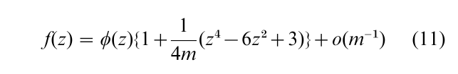
where φ(z) is the standard normal density function, and the constant is adjusted so that the area under the curve is one. (Since the t distribution is symmetric around the origin, the O(1/√ m) term does not appear in the right-hand side of the equation.) Rewriting in terms of X, the asymptotic expansion of the t statistic with m degrees of freedom is

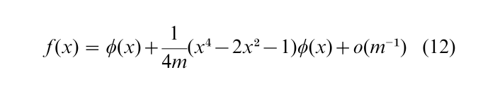
The first term in the right-hand side is the n(0, 1) density function. The second term in the right-hand side converges to zero if the limit is taken with respect to m. This second term gives deviation of f (x) from φ(x), and is called the third-order term. For finite m, the third-order term is expected to improve the standard normal approximation. The numerical evaluation of this expansion is easy.

The asymptotic expansions in the simultaneous equation estimators are long and include nuisance parameter matrices such as q below. See Phillips (1983) for a review and Phillips (1977) for the validity of expansion. The asymptotic expansion does not require the assumption of the normal distribution of the error term. Fujikoshi et al. (1982) gave the expansion of the joint density of the estimators of δ_i. In their study, the bias of the estimators is calculated from the asymptotic expansions as

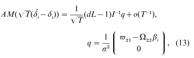
where δ is the estimator, d is 1 and 0 fo1r 2SLS and LIML estimators, respectively, and the Ω matrix is partitioned into submatrices conformable with the partitions of G and C matrices. AM(•) stands for the mean operator, but uses the asymptotic expansion for the density function. (Recall that the exact mean does not exist in the LIML estimator.) It is possible to compare the two estimators in terms of the calculated bias. For example, the bias of the 2SLS estimator is 0 when the degree of overidentifiability L is 1.

Further, the mean of the squared errors was calculated from the asymptotic expansions and used to compare estimators. It was proved that the mean squared error of the 2SLS estimator is smaller than that of the LIML estimator when L is less than or equal to 6. Historically, this kind of comparison of ‘approximate’ mean squared errors goes back to the ‘Nagar expansion’ by Nagar (1959) and the ‘small disturbance expansion’ by Kadane (1971). These qualitative comparisons gave researchers some guidance about the choice of estimators.

It was interesting to examine the accuracy of the approximations calculated by the asymptotic expansions of distributions. If the asymptotic expansions were accurate, calculation of the exact distributions could be avoided, and properties of estimators could be found easily from the approximations. However, the approximations were found not to be accurate enough to replace the exact distributions. There are many cases where the asymptotic expansion is accurate when the asymptotic distribution, the first term in the expansion, is already accurate; the asymptotic expansion is inaccurate when the asymptotic distribution is inaccurate. In particular, the asymptotic expansions are inaccurate when

(a) The value of asymptotic variance is small;

(b) The value of L is large; or

(c) The structural error term is highly correlated with the right-hand side endogenous variable.

It is noted, first, Z´Z/T is assumed to converge a nonsingular fixed matrix in the asymptotic theory. Second, for an attempt to improve the accuracy of asymptotic distributions by incorporating large L values, see Morimune (1983). Third, the asymptotic expansions cannot trace closely the skewed exact distributions that happen particularly when the correlation is high.

6. Higher-Order Efficiency Of The System And The Single-Equation Estimators

The asymptotic expansions of distributions can be used in comparing the probabilities of concentration of estimators about the true parameter values. One estimator is more desirable than another if its probability is greater than that of the other. This measure was used in comparing the single-equation estimators, and some qualitative results were derived.

Furthermore, the third-order efficiency criterion was brought in the comparisons. This criterion requires that estimators be adjusted to have the same asymptotic bias as in Eqn. (13). Then the adjusted estimators are compared, and the maximum likelihood estimator is proved most efficient. It has the highest concentration about the true parameter values in terms of the asymptotic expansion of distribution to the third-order O(1/T) terms. (Akahira and Takeuchi (1981), for example.) The adjusted maximum likelihood estimator has the smallest mean-squared error at the same time since the difference among estimators is found only in the mean-squared errors.

In whole system estimation, the FIML estimator is third-order efficient. The 3SLS estimator is less efficient than the FIML estimator in terms of the asymptotic probability of concentration once the bias of the two estimators is adjusted to be the same. Morimune and Sakata (1993) derived a simple adjustment of the 3SLS estimator so that the adjusted estimator has the same asymptotic expansion as the FIML estimator to the third-order O(1/T) terms. This estimator is explained by modifying Eqn. (7) . In Eqn. (6), Yi is replaced by Y_i = Z Π_i = Z(Z´Z)⁻¹ Z´Y_i so that the X matrix consists of Z´Y_i and Z´Z_i. In the modified estimator, we estimate Σ and Π by the first round 3SLS estimator and replace Y_i in X by Y_i = ZΠ_i where Π_i consists of proper subcolumns in Π = ΓB⁻¹. The new X matrix is denoted as X. Finally, the new estimator is

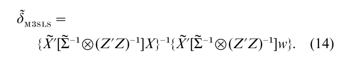
This estimator has the same asymptotic expansion as the FIML estimator to the third-order terms and is third-order efficient.

The LIML and 2SLS estimators are simple cases of the FIML and 3SLS estimators, respectively. Then the modified 2SLS estimator which follows from Eqn. (14) has the same asymptotic expansion as the LIML estimator to the third-order term. The LIML estimator and the modified 2SLS estimator are third-order efficient in the single-equation estimation.

7. Conclusion

Laurence Klein received the 1980 Nobel prize for the creation of a macroeconometric model which is an empirical form of a simultaneous equation system, and for the application to the analysis of economic fluctuations and economic policies. The macroeconometric model became a standard tool to analyze the economies and policies of nations. Trygve Haavelmo received the 1989 Nobel prize for his contribution in the analysis of simultaneous structures. Haavelmo, together with other researchers at the Cowles Commission for Research in Economics, then at the University of Chicago, became the founders of simultaneous equation analysis in econometrics. Part of their research is collected in Hood and Koopmans (1953). Studies on the exact and approximate distributions of estimators came after the research conducted at the Cowles group, and helped to make econometrics rigorous.

Access to computers was the main concern when econometric model-building started spreading all over the world in the 1970s. Since then, computer facilities surrounding econometric model-building have changed greatly. Bulky mainframe computer have been replaced by personal computers. Computer programs were written individually, mostly in Fortran, and were used for regression analyses in model estimation as well as for simulation studies in econometrics theory. The packaged least squares programs replaced the individually written programs later in model estimation. They run on personal computers and have facilitated greatly the conducting of empirical studies.

Bibliography:

1. Akahira M, Takeuchi K 1981 Asymptotic Efficiency of Statistical Estimators: Concepts and Higher Order Asymptotic Effi Springer, New York
2. Anderson T W 1958 An Introduction to Multivariate Statistical Analysis. Wiley, New York
3. Anderson T W, Rubin H 1949 Estimation of the parameters of a single equation in a complete system of stochastic equations. Annals of Mathematical Statistics 20: 46–63
4. Anderson T W, Kunitomo N, Sawa T 1982 Evaluation of the distribution function of the limited information maximum likelihood estimator. Econometrica 50: 1009–27
5. Basmann R L 1957 A generalized classical method of linear estimation of coefficients in a structural equation. Econometrica 25: 77–83
6. Cragg J G 1967 On the relative small sample properties of several structural equation estimators. Econometrica 35: 89–110
7. Fujikoshi Y, Morimune K, Kunitomo N, Taniguchi M 1982 Asymptotic expansions of the distributions of the estimates of coefficients in a simultaneous equation system. Journal of Econometrics 18: 191–205
8. Hood W C, Koopmans T C 1953 Studies in Econometric Methods. Wiley, New York
9. Kadane J B 1971 Comparison of k-class estimates when the disturbance is small. Econometrica 39: 723–37
10. Kinal T W 1980 The existence of moments of k-class estimators. Econometrica 48: 241–9
11. Mariano R S, Sawa T 1972 The exact finite sample distribution of the limited information maximum likelihood estimator in the case of two included endogenous variables. Journal of the American Statistical Association 67: 159–63
12. Morimune K 1983 Approximate distributions of k-class estimators when the degree of over-identifiability is large compared with the sample size. Econometrica 51: 821–41
13. Morimune K, Sakata S 1993 Modified three stage-least squares estimator which is third-order effi Journal of Econometrics 57: 257–76
14. Nagar A L 1959 The bias and moment matrix of the general kappa-class estimators of the parameters in simultaneous equations. Econometrica 27: 575–95
15. Phillips P C B 1977 The general theorem in the theory of asymptotic expansions as approximation to the finite sample distributions of econometric estimators. Econometrica 45: 1517–34
16. Phillips P C B 1983 Exact Phillips. In: Griliches Z, Intriligator M D (eds.) Handbook of Econometrics. North-Holland, Amsterdam, Vol. 1, Chap. 8
17. Phillips P C B 1985 The exact distribution of LIML: 2. International Economic Reviews 25(1): 249–61
18. Press S J 1982Applied Multivariate Analysis: Using Bayesian and Frequentist Methods of Inference [original edn. 1972, 2nd edn.] Robert E Krieger, Malabar, FL
19. Theil H 1961 Economic Forecasts and Policy, 2nd edn. NorthHolland, New York, pp. 231–2, 334–6
20. Zellner A, Theil H 1962 Three-stage least squares: simultaneous estimation of simultaneous equations. Econometrica 30: 54–78