Factor Analysis And Latent Structure Research Paper

Indeed, a latent variable problem can be regarded as a standard statistical problem in which the data on the latent variables are missing. There is no essential difference, for purposes of analysis, between a problem in which some of the data are never obtained and one in which some are lost.

1. Introduction

Latent variables arise mainly, but not exclusively, in the social sciences. This is because social science often deals in concepts which are constructs rather than the directly measurable variables which are typical of physical sciences. The earliest example, and still one of the most important, is general intelligence or ‘g.’ This goes back to Spearman (1904) and was constructed to describe the variation among individuals in what appeared to be common to a wide range of mental tests. Psychology and sociology abound in such latent variables. Attitudes as well as abilities are all spoken of in the discourse of these subjects as things which occur in varying amounts and which, therefore, appear in the theory as quantitative variables. In economics, variables like business confidence play a similar role. It could be justly claimed that the aspiration of these subjects to be regarded as sciences depends on the success with which latent variables can be quantified.

Latent variables can be classified into several types. Many, like intelligence, are conceived of as continuous in which case we are looking for a scale on which individuals can be located. In other contexts it is more appropriate to think of the latent variable as categorical. In that case individuals are supposed to belong to one of several classes which may or may not be ordered. What is true of the latent variables is, of course, true for the manifest variables and the only essential difference between the various methods is in the types of variables for which they are appropriate.

A convenient way of displaying the relationship between the methods is to introduce the fourfold classification of Table 1. We classify the manifest and the latent variables as metrical or categorical. In the former case we mean that they take values on some continuous or discrete scale of measurement; in the latter, that they fall into categories.

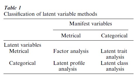
This classification is not exhaustive. It does not, for example, include cases where both kinds of variable occur among the manifest (or latent) variables. Neither does it distinguish between continuous and discrete metrical variables or between ordered and unordered categorical variables. Nevertheless, it does cover the most widely used methods on which this overview focuses.

2. Historical Perspective

Factor analysis was invented by Spearman (1904) for the specific purpose of operationalizing the notion of general intelligence. He remained wedded to the view that there was a single dominant latent variable of human ability which he named ‘g’ which accounted for most of the variation in observed performance. Thurstone (1947) emphasized the multifactorial approach and, for that purpose, generalized Spearman’s treatment to allow for several factors. Factor analysis was ahead of its time in two senses. First, it was a sophisticated multivariate technique introduced long before the statistical technology required was available. In consequence, its development was somewhat idiosyncratic and its separation from the statistical mainstream gave it an alien appearance which persists to this day and still causes suspicion and misunderstanding. Second, it is a computer intensive technique whose full potential could only be realized with the arrival of the powerful electronic computers since the 1980s. This lack distorted the early development of the subject by the need to concentrate on the search for computational shortcuts.

Latent structure analysis, which covers the remaining cells of Table 1, was introduced by Lazarsfeld after the Second World War, with a view to applications in sociology. A book-length treatment, by Lazarsfeld and Henry (1968), has held the field for many years as the definitive source of information but has now been superseded by a new generation of books of which Heinen (1996) is both recent and comprehensive.

Latent structure analysis came on the scene half a century after factor analysis, and in a different disciplinary context. For that reason there was, until very recently, little cross-fertilization between the two fields. When viewed from a level of sufficient generality, the methods are essentially the same.

In the postwar era more powerful methods became available but the whole field largely has remained a set of distinct subspecialisms each with its own literature and technology. It is over 40 years since Anderson (1959) pointed out that all latent methods shared a common conceptual framework but his insight has been slow to yield its full potential. The classification of methods as given in Table 1 was made the basis of a common approach in Bartholomew (1984) the culmination of which is to be seen in Bartholomew and Knott (1999).

3. The Basic Conceptual Framework

First, we describe the key ideas in nonmathematical terms and then, in the following section, express them more precisely. The central idea on which the treatment is based is that of a probability model in which all variables are represented by random variables. This is so natural to the modern statistician as to pass without comment, but this was not so at the time when factor analysis was being developed. Even today the notion is not always clear. A statistical model is, essentially, a statement about the joint distribution of a set of random variables. Model-building is the process of specifying that distribution.

The discussion is based on a simple example. Consider the case of arithmetical ability and suppose that this varies from one individual to another along a one-dimensional scale but cannot be observed directly. Test items are chosen which depend on this particular skill, and are administered to a large sample of subjects. Our problem is to see whether our hypothesis about the existence of a single latent variable is correct and, if so, to provide a means of locating subjects on that scale on the evidence of their test score.

A simple intuitive approach, which has been used in the educational world for generations, is to add up, or average, the scores for any individual and treat the average as an approximation to the value of the underlying latent variable for that individual. From this it is a short step to a rudimentary model according to which the observed score is equal to the ‘true score’ plus a random deviation. The deviations will tend to cancel out on addition. All latent variable models can be regarded as elaborations of this basic idea.

The first step is to specify how the observed score should vary when the value of the latent variable is fixed. The next is to deduce what the joint distribution of the scores ought to be when there is no variation. The final step is to introduce the distribution of the latent variable(s)—the true scores. Together these give the overall distribution of the scores which can then be compared with the observed distribution. If the two are in agreement the model is supported, if not it must be replaced with something better.

The second stage in the model building exercise is more problematical. By definition, a latent variable can never be observed so its distribution cannot be observed either. The choice of prior distribution is thus a matter of convention. If it is chosen to be normal, that is equivalent to agreeing to adopt a scale which renders the distribution normal.

All of the models covered by Table 1 have these two elements: (a) a statement of how the scores vary when the latent variable(s) is fixed and (b) a convention about the form of the distribution of the latent variable in the population from which the sample of those tested has come. Once these two things are known probability theory provides the means to go in the reverse direction and deduce how the latent variable would vary if the observed score were to be fixed.

4. Formal Statement Of The Conceptual Framework

The last section set out the key ideas underlying all latent variable models. Here they are expressed more formally in mathematical terms. The nonmathematical reader who is interested only in specific models may pass immediately to the next section.

Denote the set of indicators by the p-vector x. Its elements x₁, x₂, …, x_p may be continuous or categorical. The latent variables are denoted by the q-vector z. In the example above there was only one latent variable, arithmetical ability, but in general, there may be several.

Any model must specify, completely or partially, the joint probability distribution of x and z denoted by f (x, z). The distinctive thing about this kind of model is that the values of z can never be observed. For this reason everything must be expressed in terms of the distribution of the observable variables x. The relationship between the two is

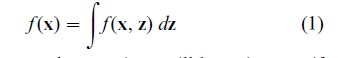
Here and subsequently equations will be written as if the variables were all continuous—hence the integral in (1). This is purely for convenience and the translation needed to cover other cases does not affect the logic of the argument. The next step is to write

decomposition provides us with the two elements to which the description of the last section referred— namely a statement of how the manifest variables would vary if z were known, given here by f (x|z), and the prior distribution of z. If both parts of (2) can be specified, f (x) can be determined and thus the way is open to estimate any parameters of the model from a likelihood function constructed from f (x). To scale z, that is to find value for z for an individual with a given x, the posterior distribution given by

is needed. A scale value, or factor score, for a particular z can then be found by using some measure of location of its posterior distribution such as E(z_i|x).

This program is deceptively simple. It merely maps out some of the consequences of regarding x and z as random variables. To turn it into a model we have to specify f (z) and f (x|z). Here we face a fundamental problem because the decomposition of (3) is not unique—there are infinitely many possible pairs each leading to the same f (x) and hence indistinguishable empirically from one another.

The choice of f (z) is resolved by appealing to the fact established above that z is a latent variable and hence that it can be constructed to have any convenient distribution. For instance, as a matter of convention one may choose the zs to be standard normal and mutually independent.

The core of the model-building exercise centers on the choice of the conditional distribution f (x|z). This has to be considered in the context of individual problems but there is one further simplification which applies to all models. This simplification involves making explicit what is already implicit in our formulation. The fact that the xs are supposed to be indicators of z implies that the xs will be mutually correlated—because of their common dependence on some, at least, of the zs. Hence, if z were to be fixed, the source of those correlations would vanish. Conditional on z the xs would then be independent. If this were not so it would be inferred that there was at least one other z, not already included, giving rise to the correlations remaining. Sufficient zs therefore have to be included in the model to eliminate the correlations after conditioning of z, It then follows that

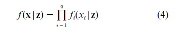
This is often referred to as the assumption of conditional (or local) independence but it is not an assumption in the usual sense. It is, rather, a statement of what is meant by saying that z explains the interdependence of the xs. It is, essentially, a definition of q as the smallest integer for which an equation of the form (4) can be constructed.

How this may be done in particular cases will be shown in the following section, but there is an important general principle which offers a fruitful way forward. Distributions of the exponential family are widely used in statistical modeling because they lead to estimates with highly desirable properties such as sufficiency. They provide a rationale for many of the most important models used in statistics, such as generalized linear models.

Essentially the same properties can be utilized here. They are set out in the chapter on the General Linear Latent Variable Models in Bartholomew and Knott (1999). The essential idea is to make what is called the ‘natural’ or ‘canonical’ parameter of the one-parameter exponential family distribution a linear function of the latent variables. If that is done it turns out that the posterior distribution of z given x of (3) depends on the xs only through q linear combinations of the xs which we may write

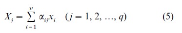
This is a remarkable result which justifies the common practice of ‘estimating’ latent variables from sums, or weighted sums, of the indicators. Technically speaking the Xs are sufficient for z in the sense that, if we know X, there is no further information in the data about z.

5. Special Cases

5.1 Factor Analysis

This is the oldest and most widely used latent variable method. It is usually written

where E(z)=E (e)=0, cov(e)=Ψ, a diagonal matrix, cov(z, e)=0 and z~N (0, I). An equivalent way of writing it, which conforms more closely to the general treatment above, is to specify the conditional distribution of x given z as

which makes it clear that z influences x only through its mean which is linear in z. The marginal distribution of x is N ( µ, ΛΛ`+Ψ) and it is from this that the parameters Λ and Ψ must be estimated. The matrix ΛΛ`+Ψ is sometimes referred to as the covariance structure.

Fitting the model consists in determining that Λ and Ψ which make the fitted and observed covariances of the xs as close as possible. This can be done without invoking the distributional assumptions at all since the covariance structure derived from (6) is the same, regardless of the assumptions about the form of the distributions of z and e. However, without some such assumption nothing can be said about goodness of fit or the sampling variation of the estimators.

Posterior analysis allows the distribution of z given x to be determined, which for the factor model is

where Σ=ΛΛ`+Ψ. As predictions of z given x we can use the mean values of this distribution, replacing the parameters by sample estimates.

5.2 Interpretation And Rotation

Interpretation of factors involves procedures which are common to all linear latent variable models. They are most familiar in the context of factor analysis so, although treated here, their generality must be emphasised. The problem may arise in two forms. If there is some idea of what factors to expect (as in the arithmetical ability example above) the question is how to recognize them. If, on the other hand, the analysis is purely exploratory, further guidance is needed on how to assign meaning to any factor that is found. The essential idea is to look at the relationships between the latent and manifest variables. This is facilitated by noting that the element λ_ij of Λ may be interpreted as the correlation between x_i and z_j. Manifest variables which are highly correlated with z say, have a lot in common with z which, in turn is highly influential in determining those xs. It must then be asked what it is that those xs have in common with one another which they also share with z . Interpretation is often facilitated by a process known as rotation. Thus far the treatment has supposed that there was only one solution to the problem of fitting the model. In fact there are infinitely many models which all predict the same covariance structure. These solutions can be generated from one another by a procedure known (because of its geometrical interpretation) as rotation. Each such solution represents an equivalent way of describing the latent space, but some may be easier to interpret than others. For example, a solution for Λ which has, at most, one nonzero value in each row implies that the xs have been divided into disjoint groups, each group depending on a single latent variable. That latent variable is then interpreted in the light of what that subset has in common.

5.3 The Latent Class Model

If the latent space consists of a finite (usually small) set of classes and if the manifest variables are also categorical the bottom right cell of Table 1 applies. The commonest case is where the manifest variables are binary. If there are c classes the prior distribution f (z) becomes a discrete probability distribution over the classes, η_j being the probability of belonging to class j. In this case these probabilities can be treated as unknown parameters to be estimated. For convenience, the two values which each x_i takes are coded as 1 and 0, the conditional distributions f_i(x_i |z) consists of two probabilities: Pr{x_i=1|z} and Pr{x_i=0|z}. The natural choice for the distribution of x_i is the Bernoulli distribution written as

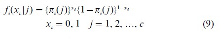
The joint probability distribution of x is then

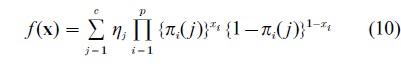
This can be used to construct the likelihood function from which the parameters may be estimated.

Posterior analysis for this case is concerned with allocating individuals to latent classes after x has been observed and this is done easily by substituting into (3). This gives us the probability that an individual with observed vector x belongs to each of the classes.

The number of parameters in this model increases rapidly with c and serious problems of identifiability arise if there are more than four or five classes. Also the standard errors of the parameter estimates increase rapidly as c increases.

5.4 Latent Trait Models

These models were devised, primarily, for use in educational testing where the latent trait refers to some ability. There is, thus, usually one latent variable, representing the ability, and many indicators. These are often binary, corresponding to the response to the item being ‘right’ or ‘wrong.’ This has become a specialized field, often referred to as Item Response Theory (IRT) with a literature and notation of its own. The model may also be used in other fields, such as sociology, where it may be more appropriate to introduce several latent variables.

A latent trait model with binary xs is similar to a latent class model. The prior distribution is now continuous and will usually be taken to be standard normal. The response variables will still be Bernoulli random variables but now they depend on the continuous latent variable(s). Since the Bernoulli distribution is a member of the exponential family the appropriate form for πi(z) turns out to be

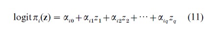
Other versions of the model in which the logit on the left hand side of (11) is replaced by Φ⁻¹(·), the inverse standard normal distribution function, are widely used and give similar results to (11) but they lack the sufficiency properties. If j=1 and the α_ijs are the same for all i, the model is a random effects version of the Rasch model (see, e.g., Bartholomew 1996). In the latter the trait values are taken as parameters rather than random variables so, in the strict sense of classical inference, the Rasch model is not a latent variable model.

5.5 Other Models

The latent profile models of Table 1 have been omitted because they have found relatively little practical application. It has also been shown by Molenaar and von Eye (1994) that they are virtually indistinguishable from factor models because they have an equivalent covariance structure. Neither have we considered hybrid models in which manifest and latent variables may be mixed type—discrete or continuous. The advantage of our general approach is that it lends itself to the treatment of all such models. This approach has been exemplified by Moustaki (1996) and is capable of further development.

6. Relationship Between Latent Variables

In much sociological research the interest is not so much in the latent variables as individual entities, but in the relationships between them. The interrelationship of manifest variables is a major subject of investigation in social science using techniques such as path analysis, regression, log-linear analysis, and graphical models. It is natural to extend these models to include latent variables. This has given rise to linear structural relations modeling which can be implemented using widely available software such as LISREL, AMOS, and EQS.

In essence, such models have two parts: (a) a measurement model which supposes that each latent variable is linked to its own set of indicators through a factor model and (b) a structural model which specifies the (linear) relationships among the latent variables. Such a model is fitted by matching the observed and theoretical covariance matrices. A much more general framework which allows a wider range of models is provided by Bartholomew and Knott (1999). Although these methods are very widely used, serious questions have been raised about the identifiability of the models (Anderson and Gerbing 1988, Croon and Bolck 1997, Bartholomew and Knott 1999). These authors have suggested that it may be better to separate the measurement and structural parts of the analysis. This can be done by constructing ‘estimates’ of the latent variables and then exploring their interrelationships by the traditional methods used for manifest variables.

7. Future Developments

The advent of massive computer power has changed the practice of multivariate analysis radically, and of latent variable analysis in particular. The limiting factor is no longer computing power but of getting data of sufficient quality and quantity to fit the very complicated models which the theory provides and computers can handle. The precision with which models with many parameters can be estimated is often very low unless the sample size runs into thousands. This makes it all the more important to estimate the sampling variability of the estimates of the parameters on which the interpretation depends. Traditionally this has been done by finding asymptotic standard errors but these can be very imprecise. However, it is now possible to supplement these results by resampling methods such as the bootstrap.

There are other fields in which latent variable models are used which currently exist in isolation. An obvious generalization is to latent time series. Some work has been done for the case where the latent process is a Markov chain. In this area the term ‘hidden’ is used instead of ‘latent’ which helps to conceal the family connections (for an introduction see MacDonald and Zucchini 1997). An application in a more traditional time series context will be found in Harvey and Chung (2000). Also, there is work by economists on unobserved heterogeneity as it is called which, essentially, involves the introduction of latent variables into econometric models.

Bibliography:

1. Anderson T W 1959 Some scaling models and estimation procedures in the latent class model. In: Grenander U (ed.) Probability and Statistics. Wiley, New York
2. Anderson J C, Gerbing D W 1988 Structural equation modeling in practice: a review and recommended two-step approach. Psychological Bulletin 103: 411–23
3. Bartholomew D J 1984 The foundations of factor analysis. Biometrika 71: 221–32
4. Bartholomew D J 1996 The Statistical Approach to Social Measurement. Academic Press, San Diego, CA
5. Bartholomew D J, Knott M 1999 Latent Variable Models and Factor Analysis, 2nd edn. Arnold, London
6. Croon M, Bolck A 1997 On the use of factor scores in structural equations models. Technical Report 97.10.102 7. Work and/organization Research Centre, Tilburg University
7. Harvey A, Chung C-H 2000 Estimating the underlying change in unemployment in the UK. Journal of the Royal Statistical Society A 163: 303–39
8. Heinen T 1996 Latent Class and Discrete Latent Trait Models: Similarities and Diff Sage, Thousand Oaks, CA
9. Lazarsfeld P F, Henry N W 1968 Latent Structure Analysis. Houghton Mifflin, New York
10. MacDonald I L, Zucchini W 1997 Hidden Marko and other Models for Discretealued Time Series. Chapman and Hall, London
11. Molenaar P C W, von Eye A 1994 On the arbitrary nature of latent variables. In: von Eye A, Clogg C C (eds.) Latent Variables Analysis: Applications for Developmental Research. Sage, Thousand Oaks, CA
12. Moustaki I 1996 A latent trait and latent class model for mixed observed variables. British Journal of Mathematical and Statistical Psychology 49: 313–34
13. Spearman C 1904 General intelligence, objectively determined and measured. American Journal of Psychology 15: 201–93
14. Thurstone L L 1947 Multiple Factor Analysis. University of Chicago Press, Chicago