Probability Density Estimation Research Paper

The same information may be obtained from the probability density function (pdf ), f(x), which equals Pr(X = x) if X takes on discrete values, or the derivative of F(x) if X is continuous. If either F(x) or f(x) is known, then any quantity of interest such as the variance may be computed analytically or numerically. Otherwise, such quantities must be estimated using a random sample x₁, x₂, …, x_n. The relative merits of estimating F(x) vs. F(x) are an important part of this research paper.

Density estimation takes two distinct forms—parametric and nonparametric—depending on prior knowledge of the parametric form of the density. If the parametric form f(x|θ) is known up to the p parameters θ = (θ₁,…, θ_p), then the parameters may be estimated efficiently by maximum likelihood or Bayesian algorithms. When little is known of the parametric form, nonparametric techniques are appropriate. The most commonly used estimators are the histogram and kernel methods, as discussed below.

1. Histograms And CDFs

Grouping and counting the relative frequency of data to form a histogram may be taught at the beginning of every statistics course, but the concept seems to have emerged only in 1662 when John Graunt studied the Bills of Mortality and constructed a crude life table of the age of death during those times of plague (Westergaard 1968). Today the histogram and its close relative, the stem-and-leaf plot, provide the most important tools for exploring and representing structure in a set of data. Studying the shape of a well-constructed histogram can verify an assumption of normality, or reveal departures from normality such as skewness, kurtosis, or multiple modes. The recent study of the theoretical properties of histograms has led to concrete methods for computing well-constructed figures as discussed below.

With only a random sample of data, the cdf may be estimated by the empirical cdf (ecdf ), denoted by F_n(x). The value of the ecdf at x is the fraction of the sample with values less than or equal to x, that is, {#x_i ≤ x}. Now the probability any one of the xi is less than x is given by the true cdf at x. Hence, on average, the value of F_n(x) is exactly F(x), and F_n(x) is an unbiased estimator of F(x). The inequality {X_i ≤ x} is a binomial random variable, so that the variance of F_n(x) may be computed as F(x)(1 – F(x))/n. In fact, there is no other unbiased estimator with smaller variance.

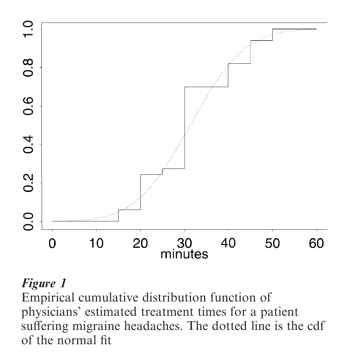
The graph of the empirical cdf looks like a staircase function. Figure 1 displays the ecdf of the treatment times estimated by 33 physicians when presented with a hypothetical patient suffering from extreme migraine headaches (Hebl and Xu 2000). The dotted line is the cdf of the fitted normal density N(31.3, 9.9²), which appears to fit reasonably well. Figure 2 displays a histogram of the same data, which does not appear to be normal after all. Social scientists often are taught to favor the ecdf over the histogram, but in fact aside from computing probabilities, the ecdf is not well- suited for the easy understanding of data.

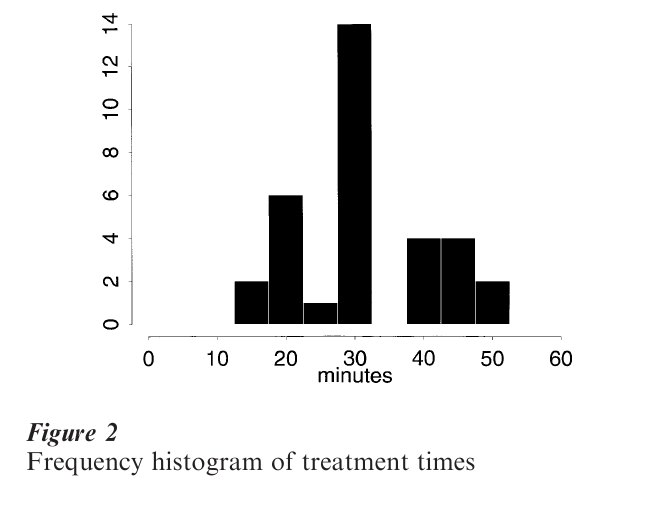
The probability density function, f (x), carries the same information as the cdf. Since the derivative of the empirical cdf F_n(x) is not well-defined, estimators that rely on grouping have been devised. A convenient interval, (a, b), containing the data is chosen, and subdivided into m ‘bins’ of equal width h = (b – a)/m. The value h is called the bin width (and is often called the smoothing parameter). A ‘well-constructed’ histogram must specify appropriate values for a, b, h, and m. Given such parameters, the number of samples falling into each of the m bins is tallied. Label the m bin counts ν₁, ν₂, …, ν_m from left to right. If the interval (a, b) contains all the samples, then Σ^m_k=1v_k=n. A frequency histogram is simply a plot of the bin counts, as in Fig. 2. Although the values are all multiples of 5 min, the data may be treated as continuous. However, the bin width should only be a multiple of 5 and care should be exercised to choose a and h so that no data points fall where two bins adjoin. Here, a = 2.5, b = 57.5, and h = 5. The histogram suggests a departure from normality in the form of three modes. Re-examine the ecdf in Fig. 1 and try to identify the same structure.

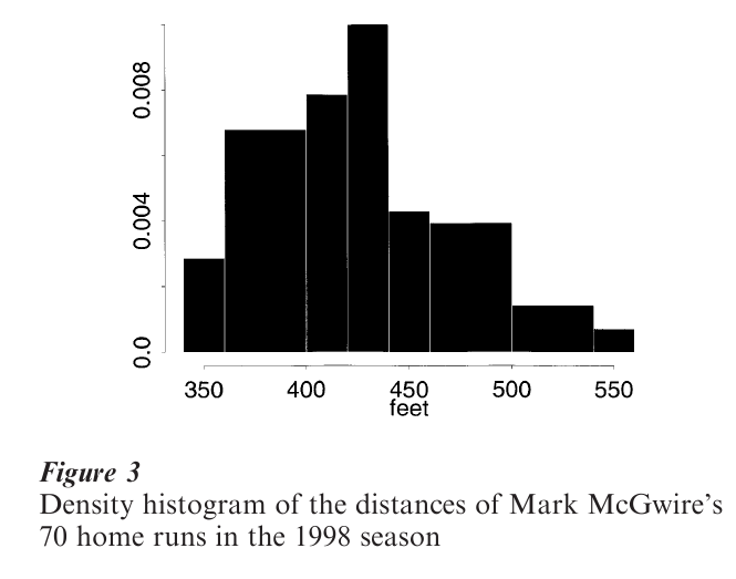
A true probability density is a non-negative function that integrates (sums) to 1. Hence, the density histogram is a simple normalization of the frequency histogram in the kth bin,

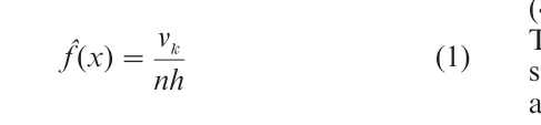
The normalization is important when the data are heavily skewed and unequal bin widths are constructed. In such cases, the interval (a, b) is partitioned into m bins of width h₁, h₂, …, h_m. The bin counts ν₁, ν₂, …, ν_m should not be plotted as they are not relatively proportional to the true density histogram, which is now given by f (x) = ν_k/(nh_k) in the kth bin. Figure 3 displays a density histogram of the distances of the 70 home runs hit by Mark McGwire during his recordsetting 1998 American baseball season. A bin width of 20 ft was chosen, and then several adjacent bins were collapsed to make the histogram look unimodal. The long right tail reflects the booming home runs for which McGwire is known.

2. Bin Width Construction

Rules for determining the number of bins were first considered by Sturges in 1926. Such rules are often designed for normal data, which occur often in practice. Sturges observed that the mth row of Pascal’s triangle, which contains the combinatorial coefficients (^m-1₀), (^m-1₁),…,(^m-1_m-1), when plotted, appears as an ideal frequency histogram of normal data. (This is a consequence of the central limit theorem for large m.) The sum of these ‘bin counts’ is 2^m-1 by the binomial expansion of (1+1)^m−1 Solving the equation n = 2^m−1 for the number of bins, we obtain Sturges’ rule This rule is widely applied in computer software.

The modern study of histograms began in Scott (1979) and Freedman and Diaconis (1981). The optimization problem formulated was to find the bin width h to make the average value of the ‘distance’ f[f(x) – f(x)]² dx as small as possible. The solution for the best bin width is

While the integral of the derivative of the unknown density is required to use this formula, two useful applications are available. First, the normal reference rule gives

since th e value of the integral for a normal density is (4√πσ³)⁻¹. The second application was given by Terrell and Scott (1985) who searched for the ‘easiest’ smooth density (which excludes the uniform density) and found that the number of bins in a density should always exceed √2n or that the bin width should always

These choices are called oversmoothed rules, as the optimal choices will never be more extreme for other less smooth densities. Notice that the normal reference rule is very close to the upper bound given by the oversmoothed rule. For the McGwire data, the over-smoothed rule gives h* ≤ 42 .

More sophisticated algorithms for estimating a good bin width for a particular data set are described in Scott (1992) and Wand (1997). For example, a cross-validation algorithm (Rudemo 1982) that attempts to minimize the error distance directly leads to the criterion

The bin counts are computed for a selection of bin widths (and bin origins), the criterion computed, and the minimizer chosen, subject to the over-smoothed bound. The criterion tends to be quite noisy and Wand (1997) describes alternative plug-in formulae that can be more stable.

All of these rules give bin widths which shrink at the rate n^−1/3 and give many more bins than Sturges’ rule. In particular, most computer programs give histograms which are oversmoothed. The default values should be overridden, especially for large datasets. Similarly, the error of the best histogram decreases to zero at the rate n^−2/3 which can be improved to n^−4/5 as described below. However, the histogram remains a powerful and intuitive choice for density estimation and presentation.

3. Advanced Algorithms

Density estimators with smaller errors are continuous functions themselves. The easiest such estimator is the frequency polygon, which connects the midpoints of a histogram. A separate error theory exists. For example, the oversmoothed bin width for a histogram from which the frequency polygon is drawn is given by

Note that this bin width is wider than the rules for the histogram alone.

Many other estimators exist, based on splines, wavelets, Fourier series, or local likelihood, but all are closely related to the kernel estimator of Rosenblatt (1956) and Parzen (1962), which is described here. The kernel can be any probability density function, but the normal density is a common and recommended choice. Here the smoothing parameter h is the standard deviation of the normal kernel. If the normal density N( µ,σ²) at a point x is denoted by φ(x|µ, σ), then the kernel estimator is

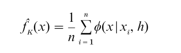
This form shows that the kernel estimator is a mixture of normal densities which are located at the data points. The oversmoothed smoothing parameter value is

An example is given below.

4. Visualization

The primary uses of density estimation are to display the structure in a set of data and to compare two sets of data. The histogram is adequate for the first task, but overlaying two histograms for comparison is difficult to interpret. The continuity and improved error properties of the kernel estimators excel for this purpose.

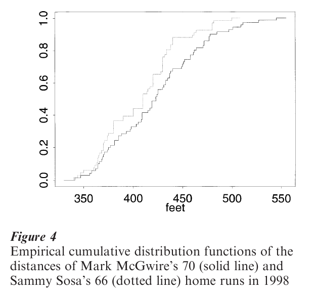
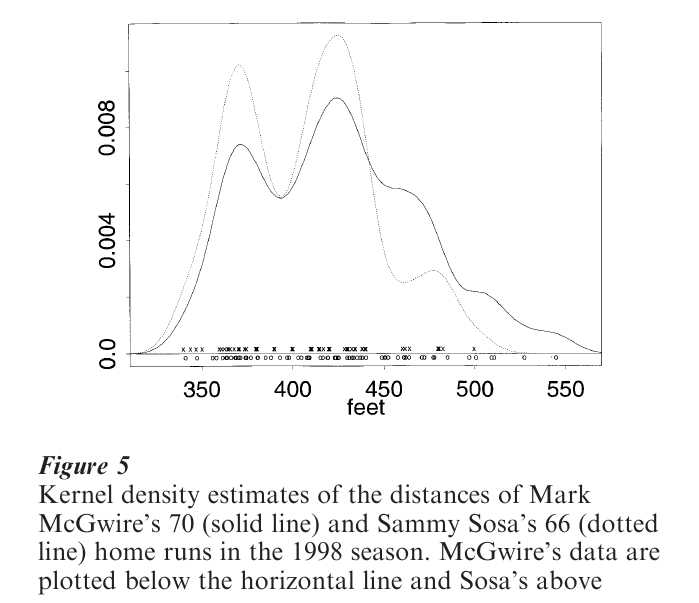
In the great home run race of 1998, Sammy Sosa finished second with 66 home runs. Figure 4 displays the empirical cdfs of the distances for the two home run kings (Keating and Scott 1999). This graph clearly shows that McGwire hits longer home runs than Sosa at every distance. In Fig. 5, kernel estimates of the McGwire and Sosa data with h 10 are overlaid. The possible structure in these data is reinforced by the similarity of the two densities. Each has two primary modes at 370 ft and 425 ft, with smaller feature around 475 ft. In addition, McGwire’s density clearly shows the right tail of his longest homers. In contrast, the modes in the original histogram of Fig. 3 did not appear convincing, and were eliminated by locally adjusting the bin widths. The continuity of the kernel and other estimators makes the assessment of modes much easier.

5. Multivariate Densities

Histograms can be constructed in the bivariate case and displayed in perspective, but cannot be used to draw contour plots. Kernel methods are well-suited for this purpose. Given a set of data (x₁, y₁), …, (x_n, y_n), the bivariate normal kernel estimator is given by

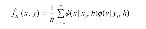
A different smoothing parameter can be used in each variable.

For three and four-dimensional data, the kernel estimator can be used to prepare advanced visualization renderings of the data. Scott (1992) provides an extension set of examples.

6. Other Materials

A number of other monographs exist that delve into various aspects of nonparametric approaches. A thorough survey of all topics by top researchers is contained in Schimek (2000). Early works popularizing these ideas include Tapia and Thompson (1978) and Silverman (1986). Wand and Jones (1994) and Simonoff (1996) focus on kernel-methods. Fan and Gijbels (1996) and Loader (1999) focus on local polynomial methods. General smoothing ideas are discussed by Hardle (1991) and Bowman and Azzalini (1997). Many other excellent references may be followed in these books.

Bibliography:

1. Bowman A W, Azzalini A 1997 Applied Smoothing Techniques for Data Analysis: The Kernel Approach with S-Plus. Clarendon Press, Oxford
2. Fan J, Gijbels I 1996 Local Polynomial Modelling and Its Applications. Chapman and Hall, London
3. Freedman D, Diaconis P 1981 On the histogram as a density estimator: L theory. Zeitschrift fur Wahrscheinlichkeitstheorie und erwandte Gebiete 57: 453–76
4. Hardle W 1991 Smoothing Techniques: With Implementation in S. Springer, New York
5. Hebl M, Xu J 2000 In: Lane D (ed.) Rice Virtual Lab in Statistics. http://www.ruf.rice.edu/lane/rvls.html
6. Keating J P, Scott D W 1999 A primer on density estimation for the great home run race of ’98 Stats 25: 16–22
7. Loader C 1999 Local Regression and Likelihood. Springer, New York
8. Parzen E 1962 On estimation of probability density function and mode. Annals of Mathematical Statistics 33: 1065–76
9. Rosenblatt M 1956 Remarks on some nonparametric estimates of a density function. Ann. Math. Statist. 27: 832–837
10. Rudemo M 1982 Empirical choice of histogram and kernel density estimators. Scandinavian Journal of Statistics 9: 65–78
11. Schimek M G (ed.) 2000 Smoothing and Regression: Approaches, Computation, and Application. John Wiley & Sons, New York
12. Scott D W 1979 On optimal and data-based histograms. Biometrika 66: 605–10
13. Scott D W 1992 Multivariate Density Estimation: Theory, Practice, and Visualization. John Wiley & Sons, New York
14. Silverman B W 1986 Density Estimation for Statistics and Data Analysis. Chapman and Hall, London
15. Simonoff J S 1996 Smoothing Methods in Statistics. Springer, New York
16. Tapia R A, Thompson J R 1978 Nonparametric Probability Density Estiamtion. Johns Hopkins University Press, Baltimore, MD
17. Terrell G R, Scott D W 1985 Oversmoothed non-parametric density estimates. Journal of the American Statistical Association 80: 209–14
18. Wand M P 1997 Dated-based choice of histogram bin width histogram. The American Statistician 51: 59–64
19. Wand M P, Jones M C 1994 Kernel Smoothing. Chapman and Hall, New York
20. Westergaard H 1968 Contributions to the History of Statistics. Agathon, New York