Statistical Clustering Research Paper

However, statistical methods can assist in classification in four ways:

(a) in devising probability models for data and classes so that probable classifications for a given set of data can be identified;

(b) in developing tests of validity of particular classes produced by a classification scheme;

(c) in comparing different classification schemes for effectiveness; and

(d) in expanding the search for optimal classifications by probabilistic search strategies.

These statistical methods are referred to as cluster analysis or statistical classification. The second term is preferred, because a cluster, from its astronomical origin, tends to connote a crowd of points close together in space, but a class is a set of objects assembled together for any kind of reason, and so the more general term classification is to be preferred. Part of the reason for the narrower term cluster analysis is that the term classification was once used in Statistics to refer to discriminant analysis. In discriminant analysis, a classification rule is developed for placing a multivariate observation into one of a number of established classes, using the joint distribution of the observations and classes. These problems are regression problems: the variable to be predicted is the class of the observations. For example, logistic regression is a method for discriminant analysis with two classes. More recently, classification in statistics has come to refer to the more general problem of constructing families of classes, a usage which has always been accepted outside of statistics.

1. Algorithms

The first book on modern clustering techniques is Sokal and Sneath (1963). The most comprehensive recent review of a huge diverse literature is Arabie et al. (1996) which includes in particular an excellent survey of algorithms by Arabie and Hubert and of probabilistic methods by Bock.

A classification consists of a set of classes; formal clustering techniques have been mainly devoted to either partitions or hierarchical clustering (see, however, the nonhierarchic structures in Jardine and Sibson 1968 and the block clusters in Hartigan 1975).

1.1 Partitions

A partition is a family of classes, sets of objects with the property that each object lies in exactly one class of the partition. Ideal-object partitions are constructed as follows. Begin with a set of given objects, a class of ideal objects, and a numerical dissimilarity between any given object and any ideal object. A fitted ideal object is associated with each class having minimum sum of dissimilarities to all given objects in the class.

The algorithm aims to determine k ideal objects, and a partition of the objects into k classes, so that the dissimilarity between an object and the fitted ideal object of its class, summed over all objects, is minimized. The usefulness of such a clustering is that the original set of objects is reduced with small loss of information to the smaller set of fitted ideal objects. Except in special circumstances, it is impracticable to search over all possible partitions to minimize the sum of dissimilarities; rather some kind of local optimization is used instead.

For example, begin with some starting partition, perhaps chosen randomly. First fit the ideal objects for a given partition. Second reallocate each object to the class of the fitted ideal object with which it has smallest dissimilarity. Repeat these two steps until no further reallocation takes place. The k-means algorithm, MacQueen (1967), is the best known algorithm of this type; each object is represented by a point in pdimensional space, the dissimilarity between any two points is squared euclidean distance, and the ideal object for each class is the centroid of the class. Asymptotic behaviour of the k-means algorithm is described in Pollard (1981).

1.2 Hierarchical Clustering

Hierarchical clustering constructs trees of clusters of objects, in which any two clusters are disjoint, or one includes the other. The cluster of all objects is the root of the tree.

Agglomerative algorithms, Lance and Williams (1967), require a definition of dissimilarity between clusters; the most common ones are maximum or complete linkage, in which the dissimilarity between two clusters is the maximum of all pairs of dissimilarities between pairs of points in the different clusters; minimum or single linkage or nearest neighbor, Florek et al. (1951), in which the dissimilarity between two clusters is the minimum over all those pairs of dissimilarities; and average linkage in which the dissimilarity between the two clusters is the average, or suitably weighted average, over all those pairs of dissimilarities.

Agglomerative algorithms begin with an initial set of singleton clusters consisting of all the objects; proceed by agglomerating the pair of clusters of minimum dissimilarity to obtain a new cluster, removing the two clusters combined from further consideration; and repeat this agglomeration step until a single cluster containing all the observations is obtained. The set of clusters obtained along the way forms a hierarchical clustering.

1.3 Object Trees

A different kind of tree structure for classification is a graph on the objects in which pairs of objects are linked in such a way that there is a unique sequence of links connecting any pair of objects. The minimum spanning tree, Kruskal (1956), is such a graph, constructed so that the total length of links in the tree is minimized. There may be more than one such optimal graph. The minimum spanning tree is related to single linkage clusters: begin by removing the largest link, and note the two sets of objects that are connected by the remaining links, continue removing links in order of size, noting at each stage the two new sets of objects connected by the remaining links. The family of connected sets obtained throughout the removal process constitutes the single linkage clusters.

In a Wagner tree, the given objects are end nodes of the tree, and some set of ideal objects are the possible internal nodes of the tree. A Wagner tree for the given objects is a tree of minimum total length in which the given objects are end nodes and the internal objects are arbitrary. A Wagner tree is a minimum spanning tree on the set of all objects and the optimally placed internal nodes. This tree has application in evolutionary biology as the most parsimonious tree reaching the given objects (Fitch and Margoliash 1967).

A third kind of tree structure arises from the CART algorithm of Breiman et al. (1984). This algorithm applies to regression problems in which a given target variable is predicted from a recursively constructed partition of the observation space; the prediction is constant within each member of the partition. If the predictors are numerical variables, the first choice in the recursion looks over all variables V and all cut- points a for each variable, generating the binary variables identifying observations where V < a. The binary predictor most correlated with the target variable divides the data set into two sets, and the same choice of division continues within each of the two sets, generating a regression tree. It is a difficult problem to know when to stop dividing. These regression trees constitute a classification of the data adapted to a particular purpose: the accurate pre- diction of a particular variable.

Usually, only the final partition is of interest in evaluating the regressive prediction, although the regression tree obtained along the way is used to decide which variables are most important in pre- diction, for example, the variables appearing in the higher levels of the tree are usually the most important. However, if there are several highly correlated variables, only one might appear in the regression tree, although each would be equally useful in prediction.

2. Probabilistic Classification

The aim is to select an appropriate classification C from some family Γ based on given data D.

2.1 Mixture Models

It is assumed that there are a number of objects, denoted x₁, …, x_n, which are to be classified. A probability model specifies the probability of an observation x when x is known to come from a class with parameter value θ, say p(x}θ). The parameter value θ corresponds to an ideal point in the partition algorithm [Sect. 1.2]. The mixture model assumes that there is a fixed number of classes k, that an object x_i comes from class C_j with mixing probability p_j, so that the probability of observation x is p(x) = Σ_j p_j p(x|θ_j), and collectively the observations have probability Π_i p(x_i). The parameters p_j and θ_j usually are estimated by maximum likelihood in a non-Bayesian approach. No single partition is produced by the algorithm, but rather the conditional probability of each partition at the maximum likelihood values of the parameters. How do these statistical partitionings compare with the dissimilarity based partitions of Sec. 1.2? Suppose the partition itself is a parameter to be estimated in the statistical model; estimate the optimal partition C = {C₁, …, C_k}, and the parameters p_j, θ_j to maximize the probability of the data given the partition Π_jΠ_xiϵCj p_j p(x_i |θ_j). Thus, the optimal partition in the statistical model is the optimal partition in a dis- similarity model with dissimilarities between the object x_i and the ideal object θ_j

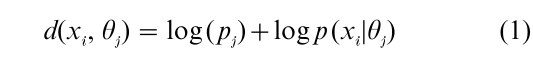
It is, thus, possible to translate back and forth between statistical models and dissimilarity models by taking dissimilarities to be log probabilities.

However, it is wrong to estimate the optimal partition by maximizing the probability of the data given the partition and parameters over all choices of partitions and parameters; as the amount of data increases, the limiting optimal partition does not correspond to the correct partition obtained when the parameters p_j, θ_j are known. (The correct partition assigns xi to the class that maximizes p_j p(x_i |θ_j). In contrast, the estimate of p_j, θ_j that maximizes the data probability averaged over all possible partitions, is consistent for the true values under mild regularity conditions, and the partition determined from these maximum likelihood estimates is consistent for the correct partition.

In a Bayesian approach, the probability model is a joint probability distribution over all possible data D and classifications C. The answer to the classification problem is the conditional probability distribution over all possible classifications C given the present data D. Add to the previous assumptions a prior distribution on the unknown parameters p_j, θ_j (Bock 1972). Again, consistent estimates of the correct classification are not obtained by finding the classification C and parameters p, θ of maximum posterior probability. Use the marginal posterior distribution of p, θ, averaging over all classifications, to give consistent maximum posterior density estimates p, θ say. Then find the classification C of optimal posterior probability C given the data and given p = p, θ = θ. This classification will converge to the optimal classification for the mixture distribution with known p and θ.

If in addition a prior distribution is specified for the number of clusters, a complete final posterior distribution is available for all possible partitions into any number of components.

2.2 Hierarchical Models

Many of the hierarchical methods assume a dissimilarity function specifying a numerical dissimilarity d(i, j) for each pair of objects i, j. If d satisfies the ultrametric inequality for every triple i, j, k

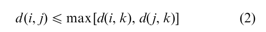
then the various hierarchical algorithms discussed in Sect. 1.2 all produce the same clusters. The dissimilarity between a given object and another object in a given cluster C is less than the dissimilarity between that object and another object not in C. Thus hierarchical clustering may be viewed as approximating the given dissimilarity matrix by an ultrametric; methods have been proposed that search for a good approximation based on a measure of closeness between different dissimilarities.

With slightly more generality, evolutionary distances between a set of objects conform to a tree in which the objects are end nodes and the internal nodes are arbitrary. A nonnegative link distance is associated with each link of the tree, and the evolutionary distance between two objects is the sum of link distances on the path connecting them. Evolutionary distances are characterised by the following property: any four objects i, j, k, l may be partitioned into two pairs of objects in three ways; for some pairing (i, j), (k, l ) say, the e olutionary equality is satisfied

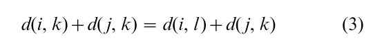
The pairing (i, j ), (k, l ) means that the tree path from i to j has no links in common with the tree path from k to l. We can construct an evolutionary tree on a set of objects by approximating a given dissimilarity by an evolutionary distance.

One case where evolutionary distances arise probabilistically is in the factor analysis model in which the objects to be classified form a set of variables on which a number of independent -dimensional observations have been made (Edwards and Cavalli-Sforza 1964). The variables are taken to be end-nodes in an evolutionary tree whose links and internal objects remain to be determined. Associated with each link of the tree is an independent normal variable with mean zero and variance depending on the link; this variance is the link distance. Each observation for the v variables is generated by assigning the random link values; then the variable V_i – V_j is a sum of independent normal variables along the path of directed links connecting i and j. The random normal associated with each link is of opposite sign when the link is traversed in the opposite direction. The quantities d(i, j ) = E(V_i – V_j)² form a set of evolutionary distances, which are estimated by d(i, j) = sample have (V_i – V_j)².

For each observation {V₁ – V_i, i = 2, … p} is multivariate normal with a covariance matrix determined by the link variances, and the log likelihood may be written, for a certain weight function w

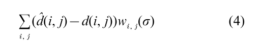
This expression is maximized to estimate the unknown σ values. In this case the sample distances form a sufficient statistic for the parameters, and no information is lost in using distances rather than the complete data set. Similar discrete Markovian models due to Felsenstein (1973) reconstruct evolutionary trees from DNA sequence data.

A nonparametric model for hierarchical clustering assumes that the objects x₁, …, x_n to be clustered are sampled randomly from a space with values x ϵ S and density f with respect to some underlying measure, usually counting measure or lebesgue measure. It is necessary to have a concept of connectedness in the space S. The family of connected sets of points having density f (x) > c, computed for each nonnegative c, together form a hierarchical clustering called high density clusters (Bock 1974, Hartigan 1975). The statistical approach estimates this hierarchical clustering on the density f from the given sample x₁, …x_n by first estimating the density f by f say, then forming the estimated clusters as the high density clusters in f. There are numerous parametric and nonparametric estimates of density available.

How do the standard hierarchical clustering methods do in estimating these high density clusters Badly. The single linkage clusters may be re-expressed as the high density clusters obtained from the nearest- neighbor density estimator; the density estimate at point x is a decreasing function of d(x, x_i), where x_i is the closest sample point to x. This estimator is inconsistent as an estimate of the density, and the high density clusters are correspondingly poorly estimated. However, it may be shown that the single linkage method is able to consistently identify distinct modes in the density. On the other hand, complete linkage corresponds to no kind of density estimate at all, and the clusters obtained from complete linkage are not consistent for anything at all, varying randomly as the amount of data increases. In evaluating and comparing clustering methods, a statistical approach determines how well the various clustering methods recover some known clustering when data is generated according to some model based on the known clustering (Milligan 1980). The most frequently used model is the multivariate normal mixture model.

3. Validity Of Clusters

A typical agglomerative clustering produces n – 1 clusters for n objects, and different choices of dis- similarities and cluster combination rules will produce many different clusterings. It is necessary to decide ‘which dissimilarity, which agglomeration method, and how many clusters?’.

In partition problems, if a parametric mixture model is used, standard statistical procedures described in Sect. 2.1 are available to help decide how many components are necessary. These models require specific assumptions about the distribution within components that can be critical to the results. The nonparametric high density cluster model associates clusters with modes in the density. The question about number of clusters translates into a question about number of modes.

The threshold or kernel width test, (Silverman 1981), for the number of modes is based on a kernel density estimator, for example, given a measure of dissimilarity, and a threshold d, use the density estimate at each point x consisting of the sum of 1 – d(x, x_i)/d over observed objects xi within dissimilarity d of x. The number of modes in the population is estimated by the number of modes in the density estimate. To decide whether or not two modes are indicated, the quantity d is increased until at d = d , the estimated density f₁ first has a single mode. If the value d₁ required to render the estimate unimodal is large enough, then more than one mode is necessary. To decide when d₁ is large, resample from the unimodal distribution f , obtaining a distribution of resampled d₁ values for those samples, the values of d₁ in each of those resamples required to make the density estimate unimodal. The tail probability associated with the given d₁ is the proportion of resampled d₁ that exceed the given d₁. A similar procedure works for deciding whether or not a larger number of modes than 2 is justified. An alternative test that applies in 1-dimension for two modes vs. one uses the DIP statistic (Hartigan and Hartigan 1985), the maximum distance between the empirical distribution function and the unimodal distribution function that is closest to the empirical distribution function. The null distribution is based on sampling from the uniform.

4. Probabilistic Search

Consider searching for a classification C in a class Γ that will maximize l(C ) the log probability of C given the data. Γ is usually too large for a complete search, and a local optimization method is used. Define a neighborhood of classifications N(C ) for each classification C. Beginning with some initial classification C₀, steepest ascent selects C_i to be the neighbor of C_i−1 that maximizes l(C ), and the algorithm terminates at C_m when no neighbor has greater probability. Of course, the local optimum depends on the initial classification C₀, and the local optimum will not in general be the global optimum.

The search may be widened probabilistically by randomized steepest ascent or simulated annealing (Klein and Dubes 1989), as follows: rather than choosing C_i to maximize l(C ) in the neighborhood of C_i−1, choose C_i with probability proportional to exp(l(C ) /λ) from the neighborhood of C_i−1. In running the algorithm, we keep track of the highest probability classification obtained to date, and may return to that classification to restart the search. The degree of randomness λ may be varied during the course of the search. To do randomized ascent at randomness λ add to the log probability of each classification the independent random quantity -λ log E, where E is exponential; then do deterministic steepest ascent on the randomized criterion.

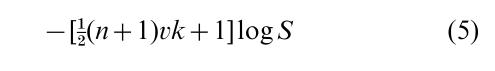
To be specific, consider the probabilification of the k-means algorithm, that constructs say k clusters of n objects in dimensions to minimize the total within cluster sum of squares S. Use a probability model in which within cluster deviations are independent normal with variance σ², the cluster mea ns are uniformly distributed, and σ² has density σ^−(2vk+4) (these prior assumptions match maximum likelihood), the log probability of a particular classification into two clusters given the data is

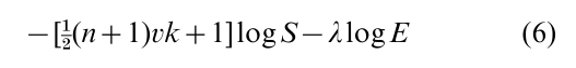
Steepest ascent k-means switches between clusters the observation that most decreases S; randomized steepest ascent switches the observation that most increases the randomized criterion

Finally, to choose the number of clusters, allowing k to vary by permitting an observation to ‘switch’ to a new singleton cluster. Penalize against many clusters by the BIC penalty; the number of parameters (cluster means and the variance) specifying k clusters in dimensions is vk + 1, so the final randomized criterion is

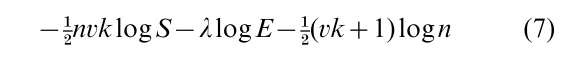
This formula adjusts only for the increase in log probability due to selecting optimal parameter values, and not for the increase in the log probability caused by selecting the highest probability partitions. A number of alternative choices of information criterion are proposed by Bozdogan (1988).

5. Conclusion

Although probabilistic and statistical methods have much to offer classification, in providing formal methods of constructing classes, in validating those classes, in evaluating algorithms, and in spiffing up algorithms, it is important to realise that classifications have something to contribute to statistics and probability as well. The early extensive development of taxonomies of animals and plants in Biology proceeded quite satisfactorily without any formal statistics or probability through 1950; the big methodological change occurred in the late-nineteenth century following Darwin, who demanded that biological classification should follow genealogy.

Classification is a primitive elementary basic form of representing knowledge that is prior to statistics and probability. Many of the standard algorithms were developed without allowing for uncertainty. Many of them, such as complete linkage, say, do not seem supportable by any statistical reasoning. Others will benefit by statistical evaluations and by probabilistic enhancements, as suggested in Hartigan (2000) and Gordon (2000).

Classification is both fundamental and subjective. If an observer classifies a set of objects to be in a class, for whatever reason, that class is valid in itself. Thus, there is no correct natural classification that our formal techniques can aim for, or that our statistical techniques can test for. Since classification is fundamental, it should be used to express formal knowledge, and probabilistic inferences and predictions should be based on these classificatory expressions of knowledge, Hartigan (2000). More formal and refined classifications may be assisted and facilitated by probability models reflecting and summarizing the prior fundamental classifications.

Bibliography:

1. Arabie P, Hubert L J, De Soete G (eds.) 1996 Clustering and Classification. World Scientific, Singapore
2. Bock H H 1972 Statistiche Modelle und Bayes’sche Verfahren zur Bestimmung einer unbekannten Klassifikation normalveteilter zufalliger Vektoren. Metrika 18: 120–32
3. Bock H H 1974 Automatische Klassifikation. Theoretische und praktische Methoden zur Gruppierung and Strukturierung on Daten (Clusteranalyse). Vandenhoek & Ruprecht, Gottingen, Germany
4. Bozdogan H 1988 A new model selection criterion. In: Bock H H (ed.) Classification and Related Methods of Data Analysis. North Holland, Amsterdam, pp. 599–608
5. Breiman L, Friedman J, Olshen R, Stone C 1984 Classification and Regression Trees. Chapman and Hall, New York
6. Edwards A W F, Cavalli-Sforza L L 1964 Reconstruction of evolutionary trees. In: Heywood V N, McNeill J (eds.) Phenetic and Phylogenetic Classification. The Systematics Association, London, pp. 67–76
7. Felsenstein J 1973 Maximum likelihood and minimum-steps methods for estimating evolutionary trees from data on discrete characters. Systematic Zoology 22: 240–49
8. Fitch W M, Margoliash E 1967 Construction of phylogenetic trees. Science 155: 279–84
9. Florek K, Lukaszewicz J, Perkal J, Steinhaus H, Zubrzycki S 1951 Sur la liaison et la division des points d’un ensemble fini. Colloquium Mathematicum 2: 282–5
10. Gordon A D 2000 Classification. Chapman and Hall, New York
11. Hartigan J A 1975 Clustering Algorithms. Wiley, New York
12. Hartigan J A 2000 Classifier probabilities. In: Kiers H A L, Rasson J-P, Groenen P J F, Schader M (eds.) Data Analysis, Classification, and Related Methods. Springer-Verlag, Berlin, pp. 3–15
13. Hartigan J A, Hartigan P M 1985 The dip test of unimodality. Annals of Statistics 13: 70–84
14. Jardine N, Sibson R 1968 The construction of hierarchic and non-hierarchic classifications. Computer Journal 11: 77–84
15. Klein R W, Dubes R C 1989 Experiments in projection and clustering by simulated annealing. Pattern Recognition 22: 213–20
16. Kruskal J B 1956 On the shortest spanning subtree of a graph and the travelling salesman problem. Proceedings of the American Mathematical Society 7: 48–50
17. Lance G N, Williams W T 1967 A general theory of classificatory sorting strategies. I: Hierarchical systems. Computer Journal 9: 373–80
18. MacQueen J 1967 Some methods for classification and analysis of multivariate observations. In: LeCam L M, Neyman J (eds.) Proceedings of the Fifth Berkeley Symposium on Mathematical Statistics and Probability. University of California Press, Berkeley, CA, pp. 281–97
19. Milligan G W 1980 An examination of the effect of six types of error perturbation on fifteen clustering algorithms. Psychometrika 45: 325–42
20. Pearson K 1984 Contributions to the mathematical theory of evolution. Philosophical Transactions of the Royal Society of London, Series A 185: 71–110
21. Pollard D 1981 Strong consistency of k-means clustering. Annals of Statistics 9: 135–40
22. Silverman B W 1981 Using kernel density estimates to investigate multimodality. Journal of the Royal Statistical Society B 43: 97–9
23. Sokal R R, Sneath P H A 1963 Principles of Numerical Taxonomy. Freeman, San Francisco