Statistical Distribution Approximations Research Paper

1. Normal Approximations

The normal or Gaussian distribution has a probability density function ( p.d.f.) given by

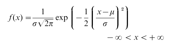
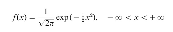
where the parameter µ is the mean or median and σ is the standard deviation. The standard normal distribution corresponds to the special case in which µ=0 and σ=1, for which the p.d.f. is given by

The normal distribution serves as an excellent approximation to many random variables that arise in nature. The reason for this lies in the central limit theorem, the simplest version of which states:

Theorem (Central limit theorem)

Suppose {X_r}^∞ _n=1 is a sequence of independent identically distributed (i.i.d.) random variables with cumulative distribution function F, mean µ, and variance σ²<∞. Then

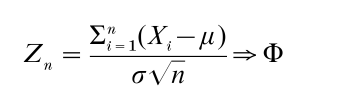
where Φ represents the c.d.f. of a standard normal distribution and → denotes weak convergence.

This theorem says that the standardized partial sums of the {X_r}^∞ _n=1 sequence converge weakly to a standard normal distribution. This theorem has many generalizations which allow for the {X_r}^∞ _n=1 to have different distributions (so long as each random variable has finite variance and contributes only a small part to the sum) and to have a dependency structure (so long as the correlation among the variables diminishes rapidly enough). The reader should consult Distributions, Statistical: Special and Continuous for additional information about the normal distribution. The textbook by DeGroot (1986) offers examples of the application of the central limit theorem, some extensions of the basic theorem, and discussions of weak convergence, also known as convergence in distribution. The reader should consult the text by Billingsley (1995) for the precisely stated theorems.

The central limit theorem indicates that suitably standardized sums of independent random variables will have an approximate normal distribution. Thus, any random variable which arises as the sum of a sufficiently large number of small random components can be modeled accurately by a normal distribution. This is especially appropriate for error distributions, where the error term is the sum of a number of different sources of error. The question of how large n must be for the approximation to be accurate depends on two factors: (a) the degree of accuracy required; and (b) the underlying distribution F. A common ‘rule of thumb’ is that the normal approximation can be safely used when n≥30 as long as F is not highly skewed and a high degree of accuracy is not required.

2. Stable Distributions

In this section, we present an extension of the central limit theorem. When {X_r}^∞ _n=1 is a sequence of i.i.d. random variables, each having a finite variance, then the partial sums of these variables can be normalized to converge weakly to a normal distribution. When the underlying random variables do not have a finite variance, then normalization of the partial sums can still lead to weak convergence to a nondegenerate limiting distribution; however, the limiting distribution will no longer be normal, but will instead be a stable distribution.

Definition (Stable distributions)

A distribution F is stable if given any three i.i.d. random variables, X₁, X₂, X₃, with distribution F and any constants c₁, c₂, there exists constants a and b (depending upon c₁, c₂) such that c₁X₁+c₂X₂ has the same distribution as a+bX₃. If a=0, the F is symmetric stable.

This means that any linear combination of two i.i.d. random variables with a common stable distribution can be transformed linearly to have the same stable distribution. This definition can be used to prove that if {X_i}ⁿ_i-1 = are i.i.d. with a stable distrinbution F, then there exist constants a_n, b_n such that Σⁿ_i=1X_i−a_n also has c.d.f. F. The symmetric stable distributions are most easily described by their characteristic functions.

Theorem (Characteristic function of a symmetric stable law)

A standard symmetric stable distribution has characteristic function φ (s)=e^−sα for 0<α≤2.

Two special cases are the normal (0,1) distribution (α=2) and the standard Cauchy distribution (α=1). The following theorem indicates that the non-degenerate stable laws represent all possible limiting distributions for sums of i.i.d. random variables.

Theorem

Suppose {X_r}^∞ _n=1 is a sequence of i.i.d. random variables with cumulative distribution function F, and suppose that there are sequenes of constants, {a_r}^∞ _n=1 and {b_r}^∞ _n=1 for which Σⁿ_i=1X_i−a_n→ G, a non- degenerate limiting c.d.f. Then G is a nondegenerate stable law.

The family of stable distributions represents a wider class of possible limits of sums of i.i.d. random variables. The distributions other than the normal have heavier tails than the normal distribution. Informally, a symmetric distribution with exponent α<2 has finite moments of order less than α. For example, the Cauchy distribution (α=1) does not have a first moment, but all moments less than 1 are finite. The stable distributions have been used to model certain economic variables and the return of financial assets such as stocks or currency exchange rates. The reader should consult Billingsley (1995), Embrechts et al. (1997), or Lamperti (1966) for more detailed information on stable distributions and the theorems underlying this more general central limit problem.

3. Extreme Value Distributions

Another type of approximation occurs when one is studying the maximum of a set of random variables. This situation is particularly relevant in the casualty insurance industry, where interest centers on the largest claims. These situations also arise in engineering and environmental problems, where a structure such as a dam or building must withstand all forces, including the largest. Suppose {X_n}^∞ _n=1 is a sequence of i.i.d. random variables with common distribution function F. Suppose that x* denotes the rightmost support point of F, the smallest x for which F (x)=1, or +∞ if no such x exists. We consider {M_n}^∞_n=1 where M_n =max_{1<i<} X_i, the largest among the first n random variables in the sequence. Fisher and Tippett (1928), a classic paper, showed that if there are sequences of constants {a_n}^∞ _n=1 and {b_n}^∞ _n=1 for which W_n-a_n/b_n→H, a nondegenerate limiting c.d.f., then H takes on one of three possible forms:

(a) The Gumbel distribution:

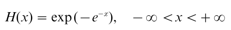
This limiting form arises when x*=∞ and the underlying distribution F has a right-hand tail which decreases at an

exponential rate. Specifically, if there exists a constant b>0 for which lim _x→∞ exp (x) (1-F(x))→b, then M_n-long(nb) converges to the Gumbel distribution as n →∞.

(b) The Frechet distribution

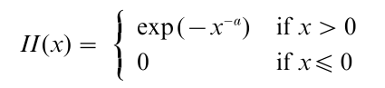
where α>0. This limiting form arises when x*=∞ and the right tail of the underlying distribution F has a tail which decays at a polynomial rate. Specifically, if lim _x→∞ x^α (1-F (x))→b , for some constant b>0 and α >0, then M_n/(bn) ^1/α converges to the Frechet distribution as n →∞.

(c) The Weibull distribution

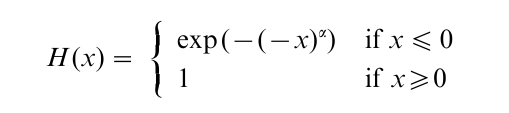
where α>0. The above distribution is concentrated on (-∞, 0), and it is the negative of the traditional Weibull distribution. This limiting form arises when x*<∞, i.e., the underlying distribution F is bounded above by a constant. Specifically, assume lim _x→x*(x*-x)^-∞ (1-F(x))→b for some constants b>0 and α>0, then (nb)^1/α (Mn-x*) converges to the Weibull distribution defined above as n→∞. The reader should consult Distributions, Statistical: Special and Continuous for additional information on the Weibull distribution.

Fisher and Tippett (1928) proved that these are the only possible limiting forms. It is, however, important to point out that, for some underlying F, there may be no set of constants {a_n}^∞ _n=1 and {b_n}^∞ _n=1 for which W_n-a_n/b_n→H. The conditions under which this convergence occurs are complicated, and the interested reader is referred to Embrechts et al. (1997). Lamperti (1966) also provides a nice treatment of extreme value theory.

The three extreme value distributions given above describe the limiting of the maximum of a random sample. There is a second random quantity that is related to the maximum and is interesting in it own right. Suppose we begin with a random variable X with c.d.f. F and consider the conditional excess distribution of X, X-u, given that it exceeds u. Specifically, consider F_u (x) =P (X-u ≤|X> u). One could also consider the expected excess, conditional on the random variable exceeding u, e (u) =E ( X -u|X -u). This distribution and expectation arise in engineering and insurance problems, where the quantity above a certain high limit is of concern, such as the insurance claim above a large deductible amount.

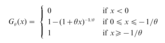
The standard generalized Pareto distribution is a family of c.d.f.s indexed by a parameter θ ϵ(-∞,+∞) given by

For θ<0,

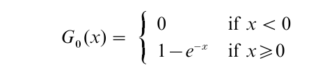
For θ=0,

For θ>0,

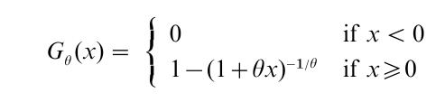
The family can be enlarged by adding a location and scale parameter.

For a given value of θ, the probability distribution of F_u approaches that of a generalized Pareto distribution as u→x*. Thus, the generalized Pareto distribution can be used to approximate the probability distribution of excesses over a high limit. The mean excesses can also be modeled using a generalized Pareto distribution.

The reader should consult Embrechts et al. (1997), a comprehensive treatment of extreme value theory and for exact conditions and statements of these approximation results.

4. Times Between Events In A Point Process

A random point process is a sequence of events (or points) that occur in time. Common examples of point processes are event histories, the failure times of systems, arrivals of customers to a service facility or the firing of neurons in the human nervous system. Clearly, modeling such point process phenomena can be very complicated and detailed. There is, however, an approximate result that is widely useful in such modeling. Specifically, for an important class of point processes, a reasonable approximation is that the times between events are i.i.d. random variables with an exponential distribution, a p.d.f. given by:

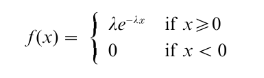
with λ>0. The parameter λ measures the rate at which the events occur and is measured in units of events per unit time. Such a point process is called a Poisson (λ) process. Poisson processes have three important properties: (a) the number of events in an interval of length L is a random variable with a Poisson (λL) distribution; (b) the number of events in non-overlapping time intervals are independent random variables; and (c) the probability of exactly one event in an interval of length h, divided by h, converges to λ as h→0. Hence events cannot occur simultaneously in a Poisson process.

Now, suppose that the point process is composed of the superposition of a large number of independent point processes, each individually with insignificant intensity function. Then the superposed (aggregated) point process converges (as the number of components superposed increases) to a Poisson process. The reader should consult the text by Karlin and Taylor (1975) for a precise statement of this theorem. This situation is very realistic for system failures in which the system is composed of many different parts, the failure of any one of which leads to system failure. Each component has its own failure distribution, and the time to the next failure will be the minimum of these failure times, which will converge to an exponential distribution as the number of components increases. A similar situation occurs with aggregate customer arrival processes, where the aggregate process is the superposition of a large number of different arrival processes. As the number of different arrival sources increases, the limiting aggregate arrival process will become Poisson. The reader should consult Queues to learn about the use of the exponential distribution, and the Poisson process as a model for customer arrival processes.

5. Further Reading

The reader should consult a basic textbook on probability such as DeGroot (1986) for information on many of the distributions mentioned in this research paper, for a description of the basic central limit theorem and examples of its use, and for some more general results. Billingsley (1995) provides a more comprehensive and technically detailed treatment of the central limit theorem, the stable laws and the extreme value distributions. Finally, the book by Embrechts et al. (1997) gives a comprehensive treatment of the extreme value distributions and associated approximation theorems.

Bibliography:

1. Billingsley P 1995 Probability and Measure, 3rd edn. Wiley, New York
2. DeGroot M H 1986 Probability and Statistics, 2nd edn. AddisonWesley, Reading, MA
3. Embrechts P, Kluppelberg C, Mikosch T 1997 Modeling Extremal Events. Springer-Verlag, Berlin
4. Fisher R A, Tippett L H C 1928 Limiting forms of the frequency distribution of the largest or smallest member of a sample. Proceedings of the Cambridge Philosophical Society 24: 180–90
5. Karlin S, Taylor H 1975 A First Course in Stochastic Processes, 2nd edn. Academic Press, New York
6. Lamperti J 1966 Probability. W. A. Benjamin, New York