Simultaneous Equation Estimation Research Paper

The simplest economic example is the interaction of buyers and sellers in a competitive market which jointly determines the quantity sold and price. Another important example is the interaction of workers, consumers, investors, firms, and government in determining the economy’s output, employment, price level, and interest rates, as in macroeconometric forecasting models. Even when one is interested only in a single equation, it often is best interpreted as one of a system of simultaneous equations.

Strotz and Wold (1960) argued that in principle every economic action is a response to a previous action of someone else, but even they agreed that simultaneous equations are useful when the data are yearly, quarterly, or monthly, because these periods are much longer than the typical market response time.

This research paper discusses the essentials of simultaneous equation estimation using a simple linear example.

1. A Simple Supply–Demand Example

Let q and p stand for the quantity sold and price of a good, y and w for the income and wealth of buyers (assumed independently determined), u₁ and u₂ for unobservable random shocks, and Greek letters for unknown constant parameters. Suppose that market equilibrium, in which the price is such that suppliers want to sell the same quantity that demanders what to buy, is described by these linear equations:

Neither equation alone can determine either p or q, because each equation contains both: these are simultaneous equations. Solve them for p and q thus:

where

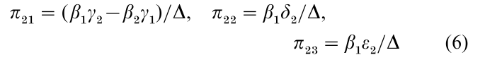
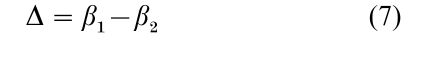
and

2. Types Of Variables: Structural And Reduced Form Equations

The variables p and q which are to be explained by the model are endogenous. Equations (1) and (2) are structural equations. Each of them describes the behavior of one of the building blocks of the model, and (as is typical) contains more than one endogenous variable. Equations (3) and (4) are reduced form equations. Each of them contains just one endogenous variable, and determines its value as a function of parameters, shocks, and explanatory variables (here y and w).

The explanatory variables are predetermined if the shocks for any given period are independent of the explanatory variables for that period and all previous periods; they are exogenous if the shocks for each period are independent of the explanatory variables for every period. Thus all exogenous variables are predetermined, but not conversely. For example, the value of an endogenous variable from a previous period cannot be exogenous, but it is predetermined if the shocks are serially independent.

3. The Need For Estimation Of Parameters

One job of a reduced form equation is to tell how an endogenous variable responds to a change in any predetermined or exogenous variable. Typically, no single structural equation can do this. Another job of a reduced form equation is to forecast the value of an endogenous variable in a future period, based on expected future values of the predetermined and exogenous variables and of the shocks (the latter can safely be set at zero in most cases). Typically, no single structural equation can do this either. If the reduced form equations are to do these jobs, numerical values of their parameters are needed (in this example, values of the πs in Eqns. (3) and (4)).

Numerical values of the structural parameters are needed as well (in this example, the βs, γs, δ₂ and ε₂ in Eqns. (1) and (2)). There are several reasons. First, one wants to understand each of the system’s separate building blocks in its own right. Second, in overidentified cases (see Sect. 7) better estimates of the reduced form can be obtained by solving the estimated structure (as in Eqns. (5)–(7) than by estimating the reduced form directly. Third, if forecasts made by the reduced form are poor, one wants to know which of the structural equations fit the forecast period’s data poorly, and which (if any) fit well. This is discovered by inserting observed values of the variables into each estimated structural equation to obtain an estimate of its forecast-period shock. Then one can revise the poorly-fitting structural equation(s) and so try to improve the model’s accuracy (see Sect. 11). Fourth, if one wants to find the new values of the reduced form parameters after a change in a structural parameter, one needs to know the old values of all the structural parameters, as well as the new value of the one that has changed. In the example, one can then use Eqns. (5)–(7) to compute the reduced form parameters. The critique of Robert Lucas (1976) provides a warning about pitfalls in doing this.

4. Least Squares Estimators

Least squares (LS) estimators of an equation’s coefficients are biased if the shocks in each period are not independent of the explanatory variables in all periods. Clearly this is true of Eqns. (1) and (2), since Eqns. (3) and (4) show that both u and u influence both p and q. This is typically true of LS estimators of simultaneous structural equations, However, LS estimators often have small variances, so they may sometimes have acceptably small expected squared errors even when they are biased.

LS estimators of the π’s in the reduced form, Eqns. (3) and (4) are unbiased if the shocks in each period have zero mean and constant variance, and are independent of y and w for all periods (so that y and w are exogenous). They have minimum variance among unbiased estimators and are consistent if in addition the shocks are uncorrelated across time. They remain consistent if the shocks are uncorrelated across time but y and w are predetermined rather than exogenous.

The generalized least squares (GLS) method is minimum variance unbiased if the explanatory variables are exogenous but the shocks are correlated across time. This method requires information about the variances and covariances of the shocks.

5. The Identifiability Of Structural Parameters

Having estimates of the reduced form parameters, one can try to make them yield estimators of the structural parameters. In the example this means trying to solve the estimated version of Eqns. (5) and (7) for estimators of the γ’s, β’s, δ₂ and ε₂. Denote the LS estimators of the π’s by π. Equations (5) and (6) show that π₂₂/ π₁₂ is one estimator of β₁, and π₂₃/π₁₃ is another. Either of them leads to an estimator of γ₁ in Eqn. (1). These are indirect least squares (ILS) estimators. They are not unbiased, but they are consistent if the LS reduced form estimators are consistent. The supply parameters β₁ and γ₁ are identified, meaning that the data and the model reveal their values (subject to sampling variation). Indeed, they are overidentified, because in small samples the two ways to estimate β₁ from π’s yield different results. (If either δ₂ and ε₂ were zero, there would be only one way, and the supply equation would be just identified. If both δ and ε were zero, there would be no way, and the supply equation would be unidentified.) Equations (5)–(7) have an infinite number of solutions for the demand parameters β₂, γ₂, δ₂ and ε₂. Hence the data and the model do not reveal their values; they are unidentified.

Another way to see this is to imagine price and quantity data being generated by intersections of the supply and demand curves in the pq plane. Ignoring shocks, the supply curve is fixed, but the demand curve shifts when y or w changes. Hence the intersections reveal the slope and position of the supply curve as the demand curve shifts. But they reveal nothing about the slope of the demand curve.

The identifiability of parameters is crucial: they cannot be estimated if they are not identified. Reduced form parameters are usually identified, except in special cases. But the identifiability of structural parameters should be checked before one tries to estimate them. The least squares formula can be applied to an unidentified structural equation such as Eqn. (2), but the result is not an estimator of that equation. For a more detailed and general discussion, see Statistical Identification and Estimability.

6. Simultaneous Equations Estimation Methods

Many methods have been developed for estimating identifiable parameters of simultaneous structural equations without the bias and inconsistency of LS. Most of them exploit the assumed independence between shocks and predetermined variables. Some estimate one equation at a time, and others estimate the whole system at once.

7. Estimating One Structural Equation At A Time

The ILS method mentioned above is one way of estimating one equation that is part of a system. A second way is the instrumental variables (IV) method (Durbin 1954). LS and IV will be shown for Eqn. (1). Denote the deviation of each variable from its sample mean by an asterisk, for example, p* = p – p. Now rewrite Eqn. (1) in terms of deviations from sample means, thus eliminating the constant term γ₁; multiply it by p*; sum it over all the sample observations; and divide the sum by ∑p*². The result is the LS estimator of β₁:

It is biased and inconsistent because the shock u influences p via Eqn. (3) so that the error term, the last term in Eqn. (8), does not equal zero in expectation or in probability limit.

Now rewrite Eqn. (1) as before in terms of deviations from sample means, but this time multiply it by y*, sum it over all observations, and divide by ∑p*y*. The result is an IV estimator of β₁:

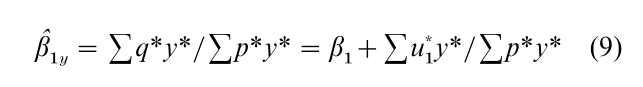
If y is predetermined it is an instrument. In this case the IV estimator is consistent if u₁ has zero mean and constant variance and is serially independent, because then ∑u*₁y* is zero in probability limit and ∑p*y* is not. Similarly, if w is predetermined it is another instrument, and another IV estimator of β₁ is β_1w = ∑q*w* / ∑p*w*. Clearly, these IV estimators are equivalent to the ILS estimators of β₁ obtained earlier. For example, the one based on the reduced form coefficients of y is

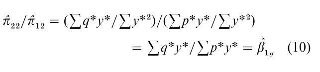
Similarly, the other one is π₂₃ /π₁₃ = β_1w. For a reduced form equation, IV is the same as LS, because the instruments are precisely the equation’s predetermined variables.

The two-stage least squares (2SLS) method (Theil 1972, Basmann 1957) is another way of estimating one structural equation at a time. For an overidentified equation it is superior to ILS or IV because it results in one estimator rather than two or more; for a just identified equation it reduces to ILS and IV. It first computes the LS estimator of the reduced form equation for each endogenous variable that appears on the right side of the structural equation to be estimated (this is stage 1); it then replaces the observed data for those endogenous variables by the values calculated from the reduced form, and computes the LS estimator for the resulting equation (this is stage 2). For Eqn. (1), stage 1 is to compute the least squares estimators of the π’s in the price equation (3) of the reduced form; the second stage is to compute p = π₁₁ + π₁₂y +π₁₃w, substitute this p for p in (1), and compute the LS estimator ∑q*p*/ ∑ p*², which is the 2SLS estimator of β₁. 2SLS is an IV estimator, its instruments are the observed values of the equation’s predetermined variables and the reduced-form-calculated values of the endogenous variables from the equation’s right side. 2SLS is a generalized method of moments (GMOM) estimator (Hansen 1982). LS and IV are plain MOM estimators.

The k-class estimator (Nagar 1959) includes as special cases LS, 2SLS, and the limited information maximum likelihood estimator (LIML) (Anderson and Rubin 1949, 1950). LIML is similar to 2SLS (the two are the same for infinitely large samples), but it has largely been displaced by 2SLS because it requires iterative computations which 2SLS does not, and because it often has a larger variance and sometimes yields outlandish estimates (Kadane 1971, Theil 1972).

For an identified structural equation, ILS, IV, LIML, and 2SLS are consistent if the model’s explanatory variables are predetermined and the shocks have zero means and constant variances and co- variances and are independent across time. An advantage of these methods is that, unlike LS, if applied to an unidentified structural equation they fail to yield estimates.

The Bayesian method of moments (BMOM) meth-od (Zellner 1998) obtains estimators of linear reduced form and structural equations without making assumptions about the likelihood function of the data. It assumes that the posterior expectations of the shocks given the data are uncorrelated with the predetermined variables, and that the differences between actual and estimated shocks have a covariance matrix of a particular form. Zellner shows how to find optimum BMOM estimators for several different loss functions, including a precision loss function which is a weighted sum of squares and cross-products of errors. For this loss function, the optimum BMOM estimator of an identified structural equation belongs to the k-class; it turns out to be LS if the ratio of the sample size to the number of predetermined variables in the model is 2, and it approaches 2SLS in the limit as this ratio grows without limit.

When a structural equation is overidentified, restrictions are placed on the reduced form parameters (such as π₂₂ / π₂₁ = π₃₂ /π₃₁ in the example, because both ratios must equal β₁), but LS estimators of the reduced form ignore this information. Better estimators of the reduced form, because they use this information, can then be obtained by solving the estimated structure (see Sect. 3).

8. Estimating A Complete System

If in an identified complete simultaneous equations system the shocks are normally distributed and other suitable conditions are satisfied, an asymptotically efficient but computationally complex method of estimating all the parameters of a complete system is the full information maximum likelihood (FIML) method (Koopmans 1950, Durbin 1988). It involves maximizing the joint likelihood function of all the data and parameters, and requires iterative computations. It has largely been displaced by the three stage least squares (3SLS) method (Zellner and Theil 1962), which is also asymptotically efficient but is much easier to compute. 3SLS is an application of the GLS method. 3SLS gets the required information on the shocks’ covariances from 2SLS estimates of the shocks; hence the name 3SLS.

9. Cross-Section vs. Time Series Studies

So far the treatment has concerned time series data, where the observations describe the same country, city, family, firm, or what not, at successive periods of time. The same type of analysis is appropriate for cross-section data, where the observations describe different countries, firms, or what not, at a single point of time, with obvious modifications. The analysis has also been extended to panel data, that is, a time series of cross-sections.

10. The Decline Of Simultaneous Equations Models

In recent years the econometric literature has paid diminishing attention to simultaneous equations models and their identifiability. Many modern textbooks give these topics little space, and that only near the end of the book (Davidson and MacKinnon 1993). Perhaps one reason is that modern computers can handle the estimation of nonlinear models, for which identification criteria are much more complicated and for which lack of identifiability is a much rarer problem.

11. The Problem Of Choosing And Testing A Model

Thus far it has been presumed that the model being estimated is an accurate representation of the real-world process that actually generates the data. This is far from certain; at best it is likely to be only approximately true. Any model has been chosen by someone, perhaps with the aid of economic theory about the maximization of profit or utility, or perhaps because it was suggested by previously observed data. But there is no guarantee that it contains the right variables, or that their endogeneity or exogeneity is correctly stated, or that the correct number of lagged variables has been chosen, or that its eqns. have the right mathematical form, or that the assumed distribution of its shocks is correct.

One can perform diagnostic tests to see whether the estimated model fits past data well, and whether its calculated past shocks have constant variance and are free of any obvious systematic behavior. But this does not assure that it will do well with future data. In my view, the most stringent and most important test of a model is to expose it to data that were not available when the model was formulated. If it does not describe these data well, it leaves something to be desired. The more new data it can describe well, the more confidence one can have in it. But at any point the best that can be said about a model is that it has done a good job of describing the data that are available thus far.

Bibliography:

1. Anderson T W, Rubin H 1949 Estimation of the parameters of a single equation in a complete system of stochastic equations. Annals of Mathematical Statistics 20: 46–63
2. Anderson T W, Rubin H 1950 The asymptotic properties of estimates of parameters of a single equation in a complete system of stochastic equations. Annals of Mathematical Statistics 21: 570–82
3. Basmann R L 1957 A generalized classical method of linear estimation of coefficients in a structural equation. Econometrica 25: 77–83
4. Christ C F (ed.) 1994 Simultaneous Equations Estimation. Edward Elgar, Aldershot, UK
5. Davidson R, MacKinnon J G 1993 Estimation and Inference in Econometrics. Oxford University Press, New York
6. Durbin J 1954 Errors in variables. Revue of the International Statistical Institute 22: 23–32
7. Durbin J 1988 Maximum likelihood estimation of the parameters of a system of simultaneous regression equations. Econometric Theory 4: 159–70
8. Haavelmo T 1943 The statistical implications of a system of simultaneous equations. Econometrica 11: 1–12
9. Haavelmo T 1944 The probability approach in econometrics. Econometrica 12(suppl.): 1–115
10. Hansen L P 1982 Large sample properties of generalized method of moments estimators. Econometrica 50: 1029–54
11. Hausman J A 1983 Specification and estimation of simultaneous equation models. In: Griliches Z, Intriligator M D (eds.) Handbook of Econometrics. North-Holland, Amsterdam, Vol. 1, pp. 391–448
12. Kadane J B 1971 Comparison of k-class estimators when the disturbances are small. Econometrica 39: 723–7
13. Koopmans T C (ed.) 1950 Statistical Inference in Dynamic Economic Models. Cowles Commission Monograph 10. Wiley, New York
14. Lucas R E Jr 1976 Econometric policy evaluation: a critique. Carnegie-Rochester Conference Series on Public Policy 1: 19–46
15. Nagar A L 1959 The bias and moment matrix of the general kclass estimators of the parameters in simultaneous equations. Econometrica 27: 575–95
16. Strotz R H, Wold H O A 1960 A triptych on causal chain systems. Econometrica 28: 417–63
17. Theil H 1972 Principles of Econometrics. Wiley, New York
18. Zellner A 1998 The finite sample properties of simultaneous equations’ estimates and estimators Bayesian and non-Bayesian approaches. Journal of Econometrics 83: 185–212
19. Zellner A, Theil H 1962 Three stage least squares: simultaneous estimation of simultaneous equations. Econometrica 30: 54–78