Stochastic Dynamic Models Research Paper

Like the classical sequential-sampling models, the main application of stochastic dynamic models is to performance in simple decision or simple information processing tasks, typically, those that require a speeded choice between two alternatives. Along with Signal Detection Theory and its variants, these models are members of a larger class of statistical decision models, which assume that the representation of stimuli in the central nervous system is inherently statistical, by virtue of the mass action properties of neural coding. This leads to models in which the stimulus representation, viewed as a sequence of events unfolding in time, is treated formally as a stochastic process.

Because of the assumed noisiness of stimulus representations, statistical decision models typically assume that decisions are made by an averaging or integration device, whose function is to smooth out transitory fluctuations in neural activation, thereby rendering decisions less susceptible to random perturbations in the stimulus process than would otherwise be the case. In Signal Detection Theory, the period of integration is assumed to be fixed, or to be determined by factors external to the stimulus process, whereas in sequential sampling models integration continues until a criterion quantity of evidence for a particular response is obtained.

From a theoretical standpoint, sequential-sampling models have greater explanatory power than signal detection models, because they can account for choice probabilities and RT within a unified theoretical framework, whereas signal-detection models provide an account of choice probabilities only. However, sequential-sampling models are more complex to analyze mathematically because they require solution of a first passage time problem. This solution gives the distribution of times needed for the accrued evidence to attain a criterion level, which is identified in such models with the decision component of RT. In contrast, the analysis of signal detection models requires only the mean and variance of the accrued evidence as a function of time, as these suffice to determine the choice probabilities.

In the sequential-sampling literature, two main classes of model have predominated: random-walk models, in which evidence accrues as a single, signed total and counter, or accumulator models, in which evidence for competing response alternatives accrues in parallel. When formulated in continuous time, these models become diffusion process models and Poisson counter models, respectively. Although a number of researchers have contributed to the development of these models, the standard versions are those described, respectively, by Ratcliff (1978) and Townsend and Ashby (1983).

Recently, dynamic generalizations of these ‘classical’ models have begun to appear, in which the assumption of a constant rate of information accrual is replaced by time-dependent accrual, state-dependent accrual, or some combination of the two. These assumptions are motivated by the need to capture the complex dynamics that seem to underlie performance in some domains. State dependence can arise when the accrual process is imperfect or ‘leaky’ (Diederich 1995, Rudd and Brown 1997, Smith 1995), or when it is governed by resistive, or approach-avoidance, dynamics (Busemeyer and Townsend 1993).

Time dependence arises when, for any of a number of reasons, the physical mechanism that generates the stimulus process is itself time varying (Heath 1992). Examples of the latter include models in which the accrual process is driven by time-varying encoding mechanisms in the visual cortex or by a noisy, continuous-time neural network, and models in which information accrual is gated in time by selective attention. In all such cases, the theoretical principles that underlie the model lead naturally to the assumption of time-dependent or state-dependent information accrual.

1. Diffusion Process Models

Figure 1 shows a two-barrier, dynamic, diffusion process model of RT. The main elements of this model are an encoding function, a source of noise, and a decision stage. The encoding function, µ(t), is a deterministic function of time, which represents the average information available to the decision stage at time t. (‘Information’ is used loosely here, to refer to the output of relevant neural systems, rather than in its technical sense of entropy.) In general, the value of µ(t) is assumed to reflect the results of an ongoing matching operation between perceptual and memorial representations of a stimulus. In Fig. 1, the encoding function arises as the difference between a time-varying stimulus representation (the continuous curve) and a sensory referent or ‘mental standard,’ c (the dashed line), which results in a function that takes on both positive and negative values. Positive values are evidence for one response, r_A; negative values are evidence for the alternative response, r_B. In classical sequential-sampling models, the encoding function is assumed to be constant for a given experimental trial ( µ(t) = µ), but in general dynamic models it may vary with time.

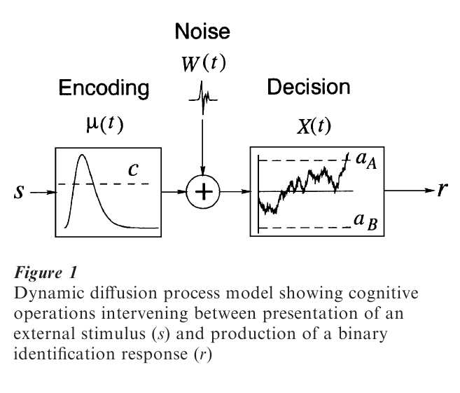
At each instant, t, the encoding function is additively perturbed by noise, W(t). In diffusion process models, the noise is assumed to be white noise, that is, broad- spectrum (delta correlated) Gaussian noise. To make a decision, successive values of the resulting noisy comparison process are integrated, as shown in the box on the right of Fig. 1. The value of the integral as a function of time is a stochastic process, X(t), which represents the accrued stimulus information at time t. The process of accrual continues until X(t) exits from the region bounded by two absorbing barriers a_A(t) and a_B(t).

If, at the time of the first boundary crossing, X(t) ≥ a_A(t), then response r_A is made; if X(t) ≤ a_B(t), then response r_B is made. Psychologically, the time of the first boundary crossing is identified with the decision time component of RT, and the probability that the first boundary crossed is a_A(t) is identified with the proportion of r_A responses. Although the figure shows a_A(t) and a_B(t) as constant, in general dynamic models the absorbing boundaries and the encoding function may all depend on time. Such variations may be useful when modeling the response to external time constraints, such as RT deadlines.

1.1 Stochastic Differential Equations For Information Accrual

In general, the process of information accrual in stochastic dynamic models can be described by a linear SDE of the form

This Eqn. defines dX(t), the random change in the accrual process X(t) in a small time interval dt. The change consists of two parts, one deterministic, the other stochastic. The deterministic change, or drift, is expressed by the quantity µ(t) + b(t)X(t). The first term µ(t), which is purely time dependent, is determined by the temporal properties of the encoding process. The second term b(t)X(t) expresses a joint dependency on time and on the current (random) state. Pure state dependency arises in the special case in which µ(t) 0 and b(t) is constant.

The stochastic part of the change, the so-called diffusion coefficient, is represented by the second term on the right of Eqn. 1. Stochastic perturbation is introduced via the white noise process, dB(t), which is the formal derivative of the Brownian motion or Wiener diffusion process. The stochastic perturbation at any instant can also be represented as the sum of two terms, one purely time dependent, σ(t), and another, c(t)X(t), that is jointly dependent on time and state. Under appropriate regularity conditions, the process X(t) that solves Eqn. 1 is a diffusion process, that is, a continuous sample path Markov process. Solutions to linear stochastic differential equations of the form of Eqn. 1 are obtained by using the Ito calculus (e.g., Karatzas and Shreve 1991).

In applications, a number of special cases of Eqn. 1 are of interest. These are instances of the case c(t) = 0, in which there is no state dependence in the diffusion coefficient. Under these circumstances, the solution to Eqn. 1 is a Gaussian process, X(t), whose distribution at time t can be characterized uniquely by its first two moments. By means of the Ito calculus it may be shown that, for a process with initial condition X(τ) = y, the value of X(t) is normally distributed with mean

and variance

These eqns. provide the basis for a dynamic signaldetection model that generalizes the classical model of Signal Detection Theory. It extends in a straightforward way to multiple correlated dimensions, to give a dynamic formulation of the General Recognition Theory of Ashby and Towsend (1986).

To date, the most important subcases of the Gaussian process in Eqns. 2 and 3 are those in which σ(t) = σ (constant) and b(t) = 0 or b(t) = γ. These subcases represent, respectively, dynamic versions of the Wiener and Ornstein-Uhlenbeck (OU) diffusion process. From a psychological perspective, the Wiener and OU processes may be thought of as describing the dynamics of stochastic accrual processes in which information integration is perfect, or ‘leaky,’ respectively.

1.2 Solution Of First Passage Time Problems For Time-Inhomogeneous Diffusions By Numerical Integral Equations

In models of RT such as the one shown in Fig. 1, the quantities of interest are the times required for X(t) to first cross one of the two absorbing boundaries, which represent decision criteria for the responses r_A and r_B. The distribution of these times are obtained by solving the first passage time problem for X(t). Classical methods for solving first passage time problems treat the problem as a boundary value problem in the theory of partial differential equations (e.g., Ratcliff 1978). However, these methods are usually not tractable when the drift term in Eqn. 1 is not time- homogeneous. Instead, such problems can often be solved using numerical integral equation techniques that were developed in mathematical biology to model the properties of integrate-and-fire neurons. These methods yield integral equation representations for g_A[a_A(t), t|x₀, t₀] and g_B[a_B(t), t|x₀, t₀], the first passage time densities of the process X(t) through the absorbing boundaries a_A(t) and a_B(t), given the initial condition X(t₀) = x₀.

To give a formal characterization of these methods, we define the transition density of X(t), the unconstrained diffusion process, by

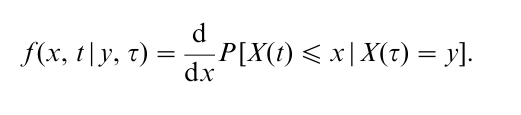
That is, the transition density is the partial derivative with respect to the spatial coordinate of the transition distribution P[X(t) ≤ x|X(τ) = y]. Classically, the transition distribution is obtained by solving the partial differential equation that is variously known as the Kolmogorov forward equation or Fokker-Planck equation, with specified initial condition. For the special Gaussian case c(t) = 0 of Eqn. 1, it may be obtained directly from the solution given by the Ito calculus, namely,

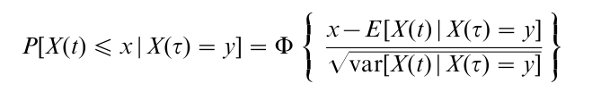
where Φ is the normal distribution function and where the moments are given by Eqns. 2 and 3.

For an arbitrary diffusion process, which may be both temporally and spatially inhomogeneous, the first passage time densities g_A[a_A(t), t|x₀, t₀] and g_B[a_B(t), t|x₀, t₀] satisfy the Fortet eqns.

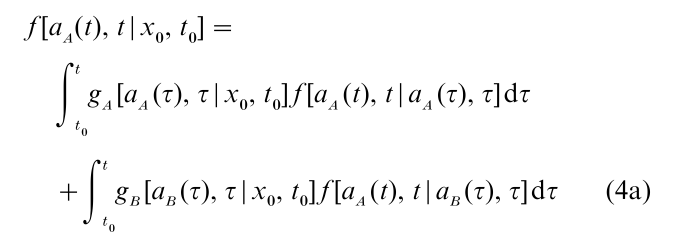
and

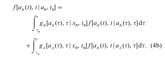
These eqns. express the unknown first passage time densities as functions of the free transition density f (x, t|y, τ) of X(t). They are obtained by considering the sample paths of X(t) that pass through one of two small open intervals a^ε_A(t) = (a_A(t), a_A(t) + ε) and a^ε_B(t) = (a_B(t), a_B(t) – ε), on the upper and lower absorbing barriers, respectively, at time t. These intervals are both in the absorbing region for X(t), so any sample path of this kind must have made at least one boundary crossing at some time τ, τ ≤ t. It may therefore be decomposed into an initial segment representing a transition from the starting point x to the point of the first boundary crossing at a_A(τ) or a_B(τ), followed by a second segment representing the subsequent transition into a^ε_A(t) or a ^ε_B(t). Because X(t) is a Markov process, the probability density for such sample paths, obtained by shrinking ε to zero, may be decomposed into a product of two density functions. One describes the first passage through an absorbing boundary at τ; the other describes the subsequent free transition (irrespective of the number of intervening boundary crossings) to a_A(t) or a_B(t). Equations 4a and 4b provide a mutually-exclusive and exhaustive decomposition of the probability densities of sample paths of this kind.

Formally, Eqns. 4a and 4b are Volterra integral equations of the first kind, which can be solved analytically only in special cases. While the general case can in principle be handled numerically, by approximating the integrals with sums, any simple method of approximation will be numerically unstable, because as the interval of approximation, h, becomes small, the transition density f (x, t|y, t – h) approaches a Dirac delta function. In the terminology of integral equation theory, the kernel of the equation is said to be singular. Consequently, recent theoretical work has sought to find ways to transform the eqn. to remove the singularity.

It was shown by Buonocore et al. (1990) and subsequently, in somewhat greater generality, by Gutierrez Jaimez et al. (1995), that for a large class of diffusion processes, Eqns. 4a and 4b can be transformed into Volterra integral equations of the second kind of the form

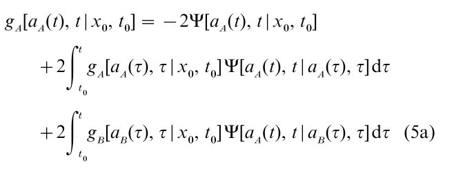
and

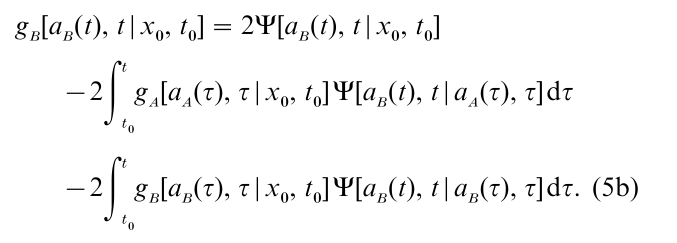
These eqns. express the first passage time densities at time t as a function jointly of their values at all preceding times, τ < t and of a kernel function Ψ(x, t|y, τ). The latter may be chosen in such a way that its value goes to zero as τ approaches t, which means that, unlike Eqns. 4a and 4b, the right-hand sides of Eqns. 5a and 5b can be approximated numerically, with finite sums. A full account of this method, including details of how to obtain the kernel functions for diffusions such as the Wiener and OU processes, may be found in Smith (2000).

1.3 Finite-State Marko Chain Approximations

Another approach to modeling decision-making using diffusion processes has been used by Busemeyer and Townsend (1992) and collaborators, in which the process is approximated numerically as the limit of a finite-state Markov chain. Computationally efficient solutions to the first passage time problem for such chains can be obtained using spectral methods when the process is time-homogeneous, as in the case of the OU process with a constant comparison function, µ(t) = µ. More recently, Diederich (1997) has extended this method to the case in which the encoding function is only piecewise time-homogeneous, that is, µ(t) = µ_i = 1, 2,…, where the index i denotes one of a sequence of consecutive, nonoverlapping observation intervals. This describes a situation in which the encoding function undergoes a sequence of instantaneous shifts during the course of an experimental trial. As such, it resembles models previously considered for piecewise random walks and Wiener processes by Ratcliff (1980) and Heath (1981), respectively. Its main application has been to model shifts in attention between stimulus attributes in cognitive decision tasks, in settings in which the time scale of the decision is long relative to that of the attention shifts. In tasks in which decisions are made more rapidly, as is the case in simple information-processing tasks, it may be more relevant to represent shifts in attention as progressive rather than instantaneous events. The dynamics of such shifts can then be modeled in continuous time using the techniques of the preceding paragraphs.

2. Poisson Counter Models

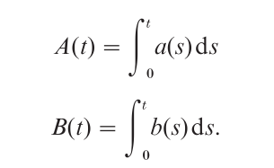
Figure 2 shows an example of the second class of stochastic, dynamic models, the Poisson parallel- counter. This model consists of three main stages: an encoding stage, a point-process generation stage, and a stochastic accrual stage. The output of the encoding stage is a function µ(t) that describes the time course of the stimulus representation. This is compared simultaneously to the mental representations of the stimuli that correspond to the response alternatives r_A and r_B. The result of this comparison is a pair of independent point processes, X_A(t) and X_B(t), whose intensities reflect the degree of the match between the stimulus and the associated mental representations. In the classical model, these stochastic comparison processes are assumed to be homogeneous Poisson processes. More generally, however, the intensities of these processes may be arbitrary functions of time, denoted a(t) and b(t). Under these circumstances, X_A(t) and X_B(t) become time-inhomogeneous.

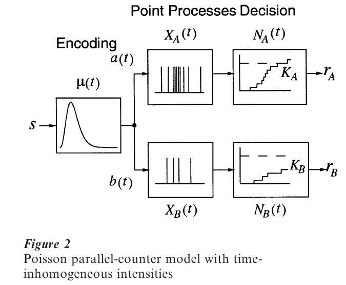
These processes drive a pair of counting processes, N_A(t) and N_B(t), which count the number of point events in X_A(t) and X_B(t), respectively. The accrual of counts continues in this way until the total in one or another counter exceeds an associated critical count, specifically, until N_A(t) ≥ K_A or N_B(t) ≥ K_B. At this point, accrual ceases and the response associated with the counter in question is given. The RT density functions for this model are determined by the integrated event rate functions A(t) and B(t), which are defined as

The first passage time densities g_A(t) and g_B(t) may then be written:

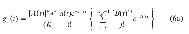
and

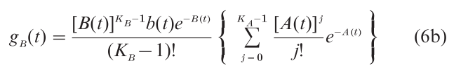
respectively. Like the time-inhomogeneous diffusion process, closed-form expressions for choice probabilities and mean RT cannot in general be obtained for this model, although these quantities may always be computed from the RT density functions by numerical integration. However, for some special cases that are of interest in applications, closed-form expressions for these statistics are readily obtainable. Details may be found in Smith and Van Zandt (2000).

3. Models With Multivariate Diffusion Processes

The preceding sections described the simplest versions of the main classes of stochastic dynamic models. However, other alternatives are possible, for example, models in which several diffusion processes race one another in parallel, as first proposed by Ratcliff (1978). Subsequent authors have considered general dynamic models in a similar vein, such as the model of simple RT described by Smith (1995), which incorporates both time inhomogeneity and state dependence. Providing the constituent processes themselves are independent, such models may be analyzed straightforwardly using the methods of Sect. 1. Usually, however, considerable complexity accompanies any attempt to relax the independence assumption in a useful way.

When the processes are not independent, their combined behavior must be modeled as a multivariate diffusion process with specified covariance properties. Distributional properties for a fairly wide variety of correlated diffusion processes may be obtained by solving the multivariate analogue of Eqn. 1 using the Ito calculus. This suffices to give the time-dependent mean and covariance function of the process, unconstrained by absorbing barriers, which provides the basis for a dynamic signal-detection model. For models of RT, however, it is usually necessary to solve the associated first passage time problem in multivariate form.

One exception to this prescription is the stochastic version of General Recognition Theory developed by Ashby (2000), which seeks to characterize how people make binary classification judgments on stimuli defined in a multivariate perceptual space. In this model, the multivariate problem can be reduced to a univariate problem because, geometrically, all the information relevant to the decision is contained in the projection of the diffusion process onto the normal to the hyper plane dividing the response categories. However, in models not possessing this structure it is necessary to solve the multivariate first passage time problem explicitly. Unfortunately, there are no general methods for solving such problems and the fragmentary results that have been obtained in special cases are usually not applicable to behavioral data. From a modeling perspective, this represents a significant limitation, because in some domains, models in which there is crosstalk between channels are of considerable theoretical interest. In these cases, because of the difficulties in obtaining relevant results in other ways, the properties of the associated models have been investigated using Monte Carlo simulation. A recent example of the use of simulation methods to investigate stochastic dynamic models is the work of Wenger and Townsend (2000).

4. Conclusions And Future Directions

This research paper has surveyed the mathematical methods used to obtain RT and accuracy predictions for the two main classes of continuous-time, dynamic models used to model decision-making in cognitive tasks: diffusion process models and Poisson parallel-counter models. The attraction of such models is that they allow richer and more complex ideas about the neural representation of stimuli to be embodied in mathematical models. The disadvantage of this additional freedom is that the resulting models may be more difficult to test empirically than their classical counterparts. For this reason, future developments in this area are likely to be in domains in which the dynamic characteristics of a model are strongly constrained by existing theory. Such constraints are needed to ensure models that are expressions of theoretical principles rather than simply vehicles for fitting data. Areas with a body of theory that is sufficiently well articulated to support models of this kind include early vision, mathematical studies of memory, and selective attention.

Bibliography:

1. Ashby F G 2000 A stochastic version of general recognition theory. Journal of Mathematical Psychology 44: 310–29
2. Ashby F G, Townsend J T 1986 Varieties of perceptual independence. Psychological Review 93: 154–79
3. Buonocore A, Giorno V, Nobile A G, Ricciardi L 1990 On the two-boundary first-crossing-time problem for diffusion processes. Journal of Applied Probability 27: 102–14
4. Busemeyer J, Townsend J T 1992 Fundamental derivations from decision field theory. Mathematical Social Sciences 23: 255–82
5. Busemeyer J, Townsend J T 1993 Decision field theory: A dynamic-cognitive approach to decision making in an uncertain environment. Psychological Review 100: 432–59
6. Diederich A 1995 Intersensory facilitation of reaction time: Evaluation of counter and diffusion coactivation models. Journal of Mathematical Psychology 39: 197–215
7. Diederich A 1997 Dynamic stochastic models for decision making under time constraints. Journal of Mathematical Psychology 41: 260–74
8. Gutierrez Jaimez R, Roman Roman P, Torres Ruiz F 1995 A note on the Volterra integral equation for the first-passagetime probability density. Journal of Applied Probability 32: 635–48
9. Heath R A 1981 A tandem random walk for psychological discrimination. British Journal of Mathematical and Statistical Psychology 34: 76–92
10. Heath R A 1992 A general nonstationary diffusion model for two choice decision making. Mathematical Social Sciences 23: 283–309
11. Karatzas I, Shreve S E 1991 Brownian Motion and Stochastic Calculus. Springer-Verlag, New York
12. Luce R D 1986 Response Times: Their Role in Inferring Elementary Mental Organization. Oxford University Press, New York
13. Pacut A 1976 Some properties of threshold models of reaction latency. Biological Cybernetics 28: 63–72
14. Ratcliff R 1978 A theory of memory retrieval. Psychological Review 85: 59–108
15. Ratcliff R 1980 A note on modeling accumulation of information when the rate of accumulation changes over time. Journal of Mathematical Psychology 21: 178–84
16. Rudd M E, Brown L G 1997 A model of Weber and noise gain control in the retina of the toad bufo marinus. Vision Research 37: 2433–53
17. Smith P L 1995 Psychophysically-principled models of visual simple reaction time. Psychological Review 102: 567–93
18. Smith P L 2000 Stochastic dynamic models of response time and accuracy: A foundational primer. Journal of Mathematical Psychology 44: 408–63
19. Smith P L, Van Zandt T 2000 Time-dependent Poisson counter models of response latency in simple judgment. British Journal of Mathematical and Statistical Psychology 53: 293–315
20. Townsend J T, Ashby F G 1983 The Stochastic Modeling of Elementary Psychological Processes. Cambridge University Press, Cambridge, UK
21. Wenger M J, Townsend J T 2000 Basic response time tools for studying general processing capacity in attention, perception and cognition. Journal of General Psychology 127: 67–99