Statistics Of Selection Bias Research Paper

1. Selection Bias

The following illustrates the basic problem. Suppose one hypothesizes the following relationship, in the population, between a dependent variable, Y*, and a set of j = 1,…, J explanatory variables, X

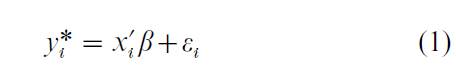
Here the unit-specific values of Y* are denoted y_i* (where i denotes the ith observation) and each unit’s values of the X variables are contained in the vector x_i. ε is a random error and the parameter vector, β, is to be estimated. Specific assumptions about the distribution of ε will determine the choice of estimation technique.

If Y* is considered as a latent variable, a variety of different statistical models can be generated from Eqn. (1) depending on the manner in which Y* is actually observed (though still, at this point, assuming that Y* is observed, in some fashion, for all units). To do this, write a second equation that defines the relationship between the observed variable Y, and the latent variable, Y*. For example, where Y* is completely observed

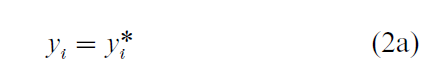
but one might also have

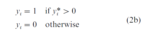
In the case of Eqn. (2(b)) Y is the binary observed realization of the underlying latent variable, Y*. More complex relationships between Y* and Y are also possible.

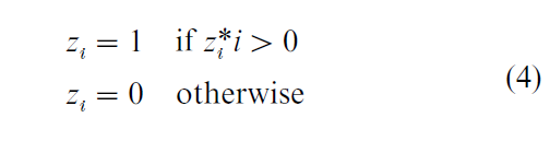
To capture the idea of selection bias, suppose that there is another latent variable Z* such that whether or not we observe a value for Y depends on the value of Z* which is given by

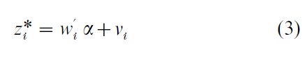
Here w is a vector of explanatory variables with coefficients α, and ν is a random error term. The observed variable Z is defined as

Finally, define the observation equation for Y as depending on Z* as follows

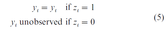
Equations (1), (2), and (5), together with Eqns. (3) and (4), link the latent variable Y* to its observed counterpart, Y, when observation of the latter depends on the value of another variable, Z*. Selection bias occurs when there is a nonzero covariance between the error terms ε and ν. More complex selection bias models can be generated by having, for instance, more than one Z* variable. The censored regression (or Tobit) model is a simpler case in which whether Y is observed or not depends on whether it exceeds (or, in other cases, falls below) a given threshold value.

2. The Problem

Selection bias is a problem because if one tries to estimate β using normal statistical methods the resulting estimates will be poor and potentially misleading. For example, if Eqn. (2(a)) specifies the relationship between Y and Y*, discarding cases where Y is unobserved and running an OLS regression on the remainder will give estimates that are biased and inconsistent.

Where might this kind of selection bias arise? Suppose one draws a random sample from a population and carries out a survey. Some respondents may refuse to answer some, though not all, questions. If the response to such a question played the role of dependent variable in a regression analysis there would be a selection bias problem if the probability of having responded to the item was not independent of the response value, given the specification of the regression model. This may not always be so: in the simplest case nonresponse might be random. Alternatively, response might be independent of the response value controlling for a set of measured covariates. In this case there is selection on observables (Heckman and Robb 1985). But often neither of these cases holds and a nonzero residual correlation between the selection Eqn. (3) and the outcome Eqn. (1) means that there is selection on unobservables.

In studies of the criminal justice system in which the population is all those charged with a crime, sentence severity is observed only for those found guilty. In studies of the effectiveness of university education the outcome (say, examination results) is only observed for those who had completed that period of education. In studies of women’s earnings in paid work the earnings of women who are not in the labor force cannot be observed. To these examples could be added very many more. Selection bias is a pervasive problem. As a consequence a variety of methods has been proposed to deal with it.

The problem of selection bias arises because of the nonzero correlation of the errors in Eqns. (1) and (3), and this arises commonly in the following context. Suppose there is a nonexperimental comparison of two groups, one exposed to some policy treatment, the other not. In this case the outcome of interest, Y, could be observed for members of both groups. Let Z now be the indicator of group membership (so that, for instance, Z = 0 means membership of the comparison group and Z = 1 means membership of the treatment group). In the case where Eqn. (2(a)) holds write the equation for Y as

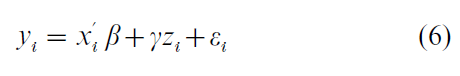
and interest would focus on the estimate of γ as the gross effect on the outcome measure of being in the treatment, rather than the comparison, group. The problem of selection bias still arises to the extent that ε and ν have a nonzero correlation. The difference between this and the type of selection bias discussed initially (namely that now Y is observed for both groups) is more apparent than real as an alternative formulation shows. For each unit Y is observed as the response to membership of either the treatment or comparison group, but not both. Let Y be the outcome given treatment and Y given no treatment. Then the ith individual unit’s gain from treatment is simply ∆_i = Y_1i–Y_0i. But ∆ cannot be measured since one cannot simultaneously observe a unit’s values of Y₁ and Y₀. Instead

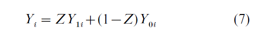
is observed. Eqn. (7) thus specifies the incomplete observation of two latent variables, Y₀ and Y₁. This set-up can easily be extended to cases with more than two groups. As might be expected, this approach is commonly encountered in the evaluation literature but one of its earliest formulations was by Roy (1951) as the problem of self-selection.

3. The Solutions

Broadly speaking there are two ways to address problems of selection bias: ex ante by research design, and ex post by statistical adjustment. The modern literature on correcting for selection bias is itself biased towards the latter, beginning with the work of Heckman in the 1970s (Heckman 1976, 1979) whose so-called ‘two step’ method is widely used and hardwired into many econometrics programs. The argument that underlies this technique is the following. Assume the set-up as defined by Eqns. (1), (2(a)), (3), (4), and (5) and a nonzero covariance between ε and ν. Then we can write the ‘outcome equation’ (i.e., the regression equation for Y, given its observability) as

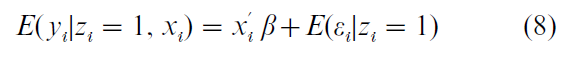
Because there are only observations of Y when z = 1 there is an extra term for the conditional expectation of ε. Because of the nonzero covariance between ε and ν and if, as is usually assumed, E(ε) = 0, then this conditional expectation cannot be zero. One can write

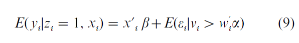
Using a standard result for the value of a truncated bivariate normal distribution, the second term on the right-hand side of this equation is given by

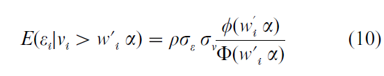
Here the σs are the standard deviations of the respective error terms from Eqns. (1) and (3); ρ is the correlation between them; φ and Φ are, respectively, the density and distribution functions of the standard normal and their ratio, as it appears in Eqn. (10), is termed the ‘inverse Mill’s ratio.’ Heckman’s two-step method requires first running a probit regression with Z as the dependent variable, estimated using all the observations in the data. Then, for those observations for which Y is observed, the probit coefficient estimates are used to compute the value of the inverse Mill’s ratio. This is then inserted as an extra variable in the OLS regression in which Y is the dependent variable to give

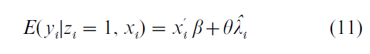
where λ is the inverse Mill’s ratio and the ‘hat’ indicates that it is estimated. Its coefficient, θ, is then itself an estimate of ρσ_εσ_ν. This is the covariance between ε and ν (σ_ν is set to unity in the probit). This approach is extended readily to the case in which an outcome is observed for both groups (Z = 0 and Z = 1).

What are the assumptions of this approach and what are the properties of the resulting estimator when we apply this method to data from a sample of the population? First, it is assumed that all the other requirements for an OLS regression are met. Second, in the set-up outlined above, the joint distribution of ε and ν should be bivariate normal (though, in general, weaker assumptions suffice, namely that ν be normally distributed; and the expectation of ε, conditional on ν, should be linear in ν: (see Olsen 1980)).

Given that the assumptions hold, the two-step estimator yields consistent estimates of the population β in Eqn. (1). The standard errors are incorrect (due to heteroscedasticity and the use of an estimated value of λ) but these are corrected readily. An alternative to the two-step approach is to estimate both the selection and outcome equations simultaneously using maximum likelihood (ML). The resulting estimates are asymptotically unbiased and more efficient than those from the two-step method (see Nelson 1984, who compares OLS, the two-step method and ML).

This two-step method is, in any case, applicable only when the relationship between Y* and Y is as given by Eqn. (2(a)). When this relationship is given by, for example, Eqn. (2(b)), the two-stage method is inconsistent. In these cases ML is the most feasible option. If the outcome variable is itself binary, the joint log-likelihood of the selection and outcome equations has the same general as for a bivariate probit but one in which there are three, rather than four, possible outcomes. They are z = 1 and y = 1; z = 1 and y = 0; and z = 0 (in which case y is not observed).

Although the two-step method is probably the most widely used approach to correcting for selection bias it has been subjected to much criticism. Among the main objections are the following:

(a) sensitivity to distributional assumptions. Practical implementation of the method renders it particularly sensitive in this respect. If the assumptions are not met the estimator has no desirable properties (i.e., it is not even consistent).

(b) identification and robustness. It is common to find that the estimate of the inverse Mill’s ratio is highly correlated either with the explanatory variables or with the intercept in Eqn. (11). The extent to which such problems will arise depends mainly on three things. They are:

(i) the specification of the selection equation;

(ii) the sample correlation between the two sets of explanatory variables, X and W (call this q);

(iii) the degree of sample selection in the sample ( p, the proportion of cases for which z = 1).

For example, if X and W are identical, the two- equation system is identified only because of the nonlinearity of the probit equation. But for some ranges of p the probit function is almost linear, with the result that the estimated λ will be close to a linear function of the explanatory variables in the probit; and thus it will be highly correlated with the X variables in the outcome equation. In general, the correlation between the inverse Mill’s ratio estimate and the other explanatory variables in this equation will be greater the greater is q and the closer is p to zero or one (this issue is discussed in detail in Breen 1996). If the selection equation does not discriminate well between the selected and unselected observations the estimated inverse Mill’s ratio will be approximately a constant, and there will therefore be a high correlation between it and the intercept of the outcome equation.

Both these objections reflect genuine difficulties in applying the model. In principle the solution to the identification and robustness problems is simple: ensure that the probit equation discriminates well and do not rely on the nonlinearity of the probit for identification. In practice it may be rather difficult to achieve these things. On the other hand, the issue of distributional assumptions may be even less tractable, obliging recourse to semiparameteric or other approaches (Lee 1994; Cosslett 1991).

An alternative is to try to assess the likely degree of bias that sample selection might induce in a given case. Rubin (1977) presents a Bayesian approach in which the investigator computes the likely degree of bias, conditional on a prior belief about the relationship between the parameters of the distribution of Y in the selected and nonselected samples. The mean and the variance of the latter sample might, for example, be expressed as a function of their values in the selected sample, conditioning on the values of observed covariates. It is then straightforward to express the extent of selection bias for plausible values of the parameters of this function and to place a corresponding Bayesian probability interval around any estimates. Rosenbaum (1995, 1996) suggests and illustrates other sensitivity analyses for selection bias in nonexperimental evaluations.

4. Program Evaluation And Selection Bias

For several years now the literature on selection bias has been dominated by discussion of how to evaluate programs (such as job training programs) when randomized assignment to treatment and control group is not possible. In a very widely cited paper, Lalonde (1986) compared the measured effectiveness of labor market programs using a randomized assignment design with their effectiveness computed using the Heckman method and showed that they led to quite different results (but see also Heckman and Hotz 1989). While some have seen this as a fatal criticism of the method, one consequence has been the development of greater awareness of the need to ensure the suitability of different selection bias correction approaches for specific cases. Another has been a greater concern to identify other possible sources of bias in nonrandomized program evaluations.

In the statistical literature, matching methods commonly are advocated in program evaluations in the absence of randomization. They involve the direct comparison of treated and untreated units that share common, or very similar, values on a set of relevant covariates, X. The rationale for this is the assumption that, conditional on X, and assuming only selection on observables (all of which are in X ), the observed outcome for nonparticipants has the same distribution as the unobserved outcome that participants would have had had they not participated (see Heckman et al. 1997). This then allows one to estimate ∆. In passing, note that matching is also used commonly to impute missing values in item nonresponse in surveys (Little and Rubin 1987). A central issue is how to carry out such matching. If there are K covariates, then the problem is one of matching pairs, or sets, of participants and nonparticipants in this K-dimensional space. But by a result due to Rosenbaum and Rubin (1983) (see also Rosenbaum 1995), matching using a scalar quantity called the propensity score is equally effective. The propensity score is simply the probability of being in the treatment, rather than the comparison group, given the observed covariates. Matching on the propensity score controls bias due to all observed covariates and, even if there is selection on unobservables, the method nevertheless produces treatment and comparison groups with the same distribution of X variables. This is so under the assumption that the true propensity score is known, but Rosenbaum and Rubin (1984) show that an estimated propensity score (typically using a logit model) appears to perform at least as well.

The use of matching draws attention to the problem of the possibly different distributions of covariates (or, equally, of propensity scores) in the treatment and comparison groups. There are two important aspects: first, the support of the propensity score may be different, so some ranges of propensity score values may be present in one group and not the other. More simply, some participants may have no comparable non-participants. Second, the distributions of the set of common values of propensity scores (i.e., which appear in both groups) may be different (Heckman et al. 1997, 1998). Hitherto, in practice, both of these sources of bias in evaluating the program’s effects commonly would have been confounded with selection bias proper. The use of propensity scores can remove the former but, if there is also selection on unobservables (i.e., selection bias proper), matching cannot be expected to solve the problem. Indeed, it is possible that these different forms of bias may have opposite signs, so that correcting for some but not others may make the overall bias greater. Nevertheless, the ability to draw such finer distinctions among biases is a valuable development, not least because it allows one to focus on methods for controlling selection bias, free from the contaminating effects of other biases.

5. Conclusion

This research paper has only skimmed the surface of selection bias statistics. In particular, it has looked only at models for cross-sectional data: other approaches are possible given other sorts of data. For example, given longitudinal data, with observations of Y for each unit at two (or more) points in time, one prior to the program to be evaluated, the other after it, then it may be possible to specify and test a model which assumes that unobserved causes of selection bias are unitspecific and time-invariant and can therefore be removed by differencing (Heckman and Robb 1985, Heckman et al. 1997, 1998). Considerations of this sort draw attention to the ex ante approach to dealing with selection bias that was referred to earlier. Here the emphasis falls on designing research so as to remove, or at least reduce, selection bias. Random assignment is one possibility, though not always feasible in practice. Nevertheless, quasi-experimental approaches, interrupted time-series, and longitudinal designs with repeated measures on the outcome variable are among a range of possibilities that could be considered in designing ones research to minimize selection bias problems (see Rosenbaum 1999 and associated comments). Even so, there will still be many instances in which analysts use data over whose collection they have had no control and where the use of ex post adjustments will be unavoidable.

To conclude: much work on the selection bias problem has been undertaken since the 1980s yet there is no widespread agreement on which statistical methods are most suitable for use in correcting for the problem. Some broad guidelines for practitioners can, however, be discerned:

(a) the need to ensure that methods to correct for selection bias are appropriate and that their requirements (such as distributional properties) are met;

(b) the need to be aware of other, possibly confounding, sources of bias;

(c) the usefulness of analyses of the sensitivity of conclusions to various possible magnitudes of selection bias; and of the sensitivity of the selection-bias corrected results to the assumptions of whatever method is employed; and

(d) the desirability of designing research so that selection bias problems are, as far as possible, eliminated without the need for complex and sometimes fragile ex post adjustment.

Bibliography:

1. Breen R 1996 Regression Models: Censored, Sample-selected or Truncated Data. Sage, Thousand Oaks, CA
2. Cosslett S 1991 Semiparametric estimation of a regression model with sample selectivity. In: Barnett W A, Powell J, Tauchen G (eds.) Nonparametric and Semiparametric Methods in Econometrics and Statistics. Cambridge University Press, Cambridge, UK
3. Heckman J J 1976 The common structure of statistical models of truncation, sample selection and limited dependent variables and a simple estimator for such models. Annals of Economic and Social Measurement 5: 475–92
4. Heckman J J 1979 Sample selection bias as a specification error. Econometrica 47: 153–61
5. Heckman J J, Hotz V J 1989 Choosing among alternative nonexperimental methods for estimating the impact of social programs: The case of manpower training. Journal of the American Statistical Association 84(408): 862–74
6. Heckman J J, Ichimura H, Smith J, Todd P E 1998 Characterizing selection bias using experimental data. Econometrica 66: 1017–98
7. Heckman J J, Ichimura H, Todd P E 1997 Matching as an econometric evaluation estimator: Evidence from evaluating a job training programme. Review of Economic Studies 64: 605–54
8. Heckman J J, Robb R 1985 Alternative methods for evaluating the impact of interventions. In: Heckman J J, Singer B (eds.) Longitudinal Analysis of Labor Market Data. Cambridge University Press, New York
9. Lalonde R J 1986 Evaluating the econometric evaluations of training programs with experimental data. American Economic Review 76: 604–20
10. Lee L F 1994 Semi-parametric two-stage estimation of sample selection models subject to Tobit-type selection rules. Journal of Econometrics 61: 305–44
11. Little R D, Rubin D B 1987 Statistical Analysis with Missing Data. Wiley, New York
12. Nelson F D 1984 Efficiency of the two-step estimator for models with endogenous sample selection. Journal of Econometrics 24: 181–96
13. Olsen R J 1980 A least squares correction for selectivity bias. Econometrica 48: 1815–20
14. Rosenbaum P R 1995 Obser ational Studies. Springer-Verlag, New York
15. Rosenbaum P R 1996 Observational studies and nonrandomized experiments. In: Ghosh S, Rao C R (eds.) Handbook of Statistics. Elsevier, Amsterdam, Vol. 13
16. Rosenbaum P R 1999 Choice as an alternative to control in observational studies. Statistical Science 14: 259–304
17. Rosenbaum P R, Rubin D B 1983 The central role of the propensity score in observational studies for causal eff Biometrika 70: 41–55
18. Rosenbaum P R, Rubin D B 1984 Reducing bias in observational studies using subclassification on the propensity score. Journal of the American Statistical Association 79: 516–24
19. Roy A D 1951 Some thoughts on the distribution of earnings. Oxford Economic Papers 3: 135–46
20. Rubin D B 1977 Formalizing subjective notions about the effect of nonrespondents in sample surveys. Journal of the American Statistical Association 72: 538–43