Newcomb’s Problem Research Paper

This research paper surveys the debate. The problem is stated in Sect. 1. Arguments for each of the opposed solutions are rehearsed in Sect. 2. Sect. 3 contains a sketch of causal decision theory. One strategy for defending orthodox Bayesianism is outlined in Sect. 4.

1. The Problem

There are two boxes on the table in front of you. One of them is transparent and can be seen to contain $1,000 dollars. The other is opaque. You know that it contains either one million dollars or nothing. You must decide whether to take (a) only the contents of the opaque box (call this the one-box option); or, (b) the contents of both boxes (the two-box option). You know that a remarkably accurate Predictor of human deliberation placed the million dollars in the opaque box yesterday if and only if it then predicted that you would choose today to take only the contents of that box. You have great confidence in the Predictor’s reliability. What should you do?

2. Opposed Arguments

There is a straightforward and plausible expected value argument for the rationality of the one-box choice. If you take only the contents of the opaque box, then, almost certainly, the Predictor will have predicted this and placed the million dollars in the box. If you choose to take the contents of both boxes, then, almost certainly, the Predictor will have predicted this and left the opaque box empty. Thus the expected value of the one-box choice is very close to $1,000,000, while that of the two-box choice is approximately $1,000. The one-box choice maximizes your expected value. You should therefore choose to take only one box.

But there is also a straightforward and plausible dominance argument supporting the two-box choice. The prediction was made yesterday. The $1,000,000 is either there in the opaque box or it is not. Nothing that you do now can change the situation. If the $1,000,000 is there, then the two-box choice will yield $1,000,000 plus $1,000, while the one-box choice yields only the $1,000,000. And if the opaque box is empty, there is no million dollars to be had: the two-box choice gives you $1,000, the one-box option leaves you with no money at all. Whichever situation now obtains, you will be $1,000 better off if you take both boxes. The two-box choice is your dominant option. You should therefore choose to take both boxes.

Care must be taken in applying the second argument, for dominance reasoning is appropriate only when probability of outcome is independent of choice. Example: Nasty Nephew has insulted Rich Auntie who threatens to cut Nephew from her will. Nephew would like to receive the inheritance, but, other things being equal, would rather not apologize. Either Auntie cuts Nephew from the will or she does not. If she does, Nephew receives nothing, and in this case prefers not having apologized. If she does not, then Nephew receives the inheritance, but once again, prefers inheritance with no apology to inheritance plus apology. Does a dominance argument give Nephew reason to refrain from apologizing? Clearly that line of thought is fallacious. It ignores the fact that whether or not Nephew is cut from the will may depend upon whether or not he apologizes.

Does this observation vitiate the two-boxer’s appeal to dominance? That depends on what one means by ‘dependence.’ What the Predictor did yesterday is certainly probabilistically dependent on what you choose today. The conditional probability that the opaque box contains $1,000,000 given that you choose the one-box option is close to one, while the conditional probability of the $1,000,000 being present given that you choose to take both boxes is close to zero. But yesterday’s prediction is causally independent of today’s choice, for what is past is now fixed and determined and beyond your power to influence. We are used to these two senses of dependence coinciding, but Newcomb’s problem illustrates the possibility of divergence when, for example, there is reliable information to be had about the future. Armed with the distinction, two-boxers maintain that dominance reasoning is valid whenever outcomes are causally independent of choice.

The dominance argument can be made even more vivid by considering the following variation on the original problem. The opaque box has a transparent back. Your dearest friend is sitting behind the boxes and can see the contents of both. Your friend is allowed to advise you what you should do. What choice will your friend tell you to make? Obviously: to take both boxes. Now it would be irrational to ignore the advice of a friend who has your best interests at heart and who you know is better informed than you are. And should not the fact that you know in advance what your friend would tell you to do in this variation of the problem determine your opinion about what to do in the original version?

One-boxers reply that the kind of agent who follows the friend’s advice, and two-boxers in general, will very likely finish up with only $1,000. ‘If you’re so smart’, they taunt, ‘why ain’cha rich?’ Two-boxers may counter that Newcomb’s problem is simply a situation in which one can expect irrationality to be rewarded. If ‘choosing rationally’ means no more than choosing so as to maximize expected reward, it may seem hard to see how such a response can be coherent, but see Gibbard and Harper (1978), Lewis (1981b).

3. Causal Decision Theory

Those two-boxers who are skeptical that orthodox Bayesian decision theory of the kind developed in Jeffrey (1983) can deliver the right answer to Newcomb’s problem face the challenge of providing an account of rational decision making consistent with this judgment. By the early 1980s several independently formulated but essentially equivalent versions of an alternative account had appeared. (See, for example, Cartwright (1979), Gibbard and Harper (1978), Levi (1975), Lewis (1981a), Skyrms (1982), Sobel (1978). According to this alternative account, now widely referred to as causal decision theory (CDT), calculations of expected value should be sensitive to an agent’s judgments about the probable causal consequences of the available options. The differences between this causal theory and orthodox Bayesian decision theory are perhaps best appreciated by proceeding from a definition of expected value that is neutral between the two accounts.

The notion of expected value relates the value assigned by an agent to an option A to the values the agent assigns to the more particular ways w in which A might turn out to be true. All parties to the debate agree that the expected value V(A) of an option A is a probability weighted average of the values of these various w. That is:

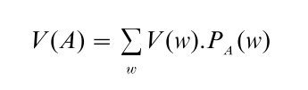
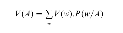
where P_A is the probability function that results when the agent’s subjective probability function P is revised so as to accept A. Where the theories differ is on the method of probability revision deemed appropriate to this context. According to the orthodox Bayesian theory, the appropriate method is revision by conditionalization on the option A:

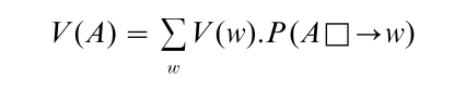
whereas causal decision theorists maintain that for each w the weight should be given by the probability of the subjunctive conditional: if A were chosen then w would be true. This conditional is usually abbreviated A□→w. Thus:

That these two definitions of expected value do not coincide is far from obvious. But in fact they do not coincide because they cannot. David Lewis, one of the co-founders of CDT, demonstrated the impossibility of defining a propositional connective □ → with the property that for each A, C the probability of the conditional A □ → C equals the conditional probability of C given A. (See Lewis (1976) and Counterfactual Reasoning, Quantitative: Philosophical Aspects and Counterfactual Reasoning, Qualitative: Philosophical Aspects.)

But the divergence of these two definitions is best seen by applying them to Newcomb’s problem. There are two options: the one-box choice (B₁) and the two-box choice (B₂); and four possible outcomes: receiving nothing (N ), receiving $1,000 (K ), receiving $1,000,000 (M ), or receiving $1,001,000 (i.e., ‘getting the lot’ L). Assume that the values you assign to these outcomes are given by the dollar amounts, and suppose finally that you have 99 percent confidence in the Predictor’s reliability, i.e., that you assign the conditional probabilities: P(M/B ) = 0.99, P(N/B₁) = 0.01, P(L/B₂) = 0.01, P(K/B₂) = 0.99.

Then on the orthodox account:

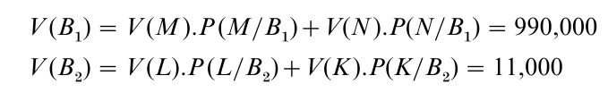
and so according to the Bayesian theory the one-box choice maximizes expected value.

Before the causal theory can be applied, probabilities must be assigned to the relevant subjunctive conditionals: B₁ □ → M, B₁ □ → N, B₂ □ → L, and B₂ □ → K. The first of these, B₁ □ → M, is the conditional: ‘If you were to take only the contents of the opaque box, then you would receive $1,000,000.’ Now this conditional is true if and only if the Predictor placed the $1,000,000 in the opaque box yesterday. Similarly the conditional B₂ □ → L: ‘If you were to take the contents of boxes, then you would receive $1,001,000’ is true just in case the Predictor put the $1,000,000 in the opaque box yesterday. It follows that:

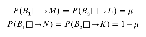
where µ is whatever probability you assign to the proposition that yesterday the Predictor placed $1,000,000 in the opaque box. Thus:

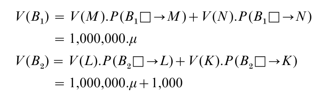
and so according to the causal theory the two-box choice maximizes expected value. Note that these assignments reflect the causal decision theorist’s advocacy of the dominance argument in a situation in which outcomes are causally independent of choice, for to say that C is causally independent of A is just to say that P(A□ → C) = P(C).

There are a couple of delicate issues involved here. First of all, one must resist the temptation to say such things as:

The $1,000,000 is there in the opaque box, but if you were to choose to take only the contents of that box, then the $1,000,000 would not be there.

A thought to which one might be led by the consideration is that:

If you were to make the one-box choice now, then the Predictor, being so reliable, would have to have predicted yesterday that that was what you would do today.

Of course these conditionals would be true if your choice today had the power to affect the past, if, for example, your choosing to take only one box could somehow cause the Predictor yesterday to have predicted that that was what you would do. But that is not so. Newcomb’s problem is not a story about backward causation. The Predictor predicted what you will do, but that prediction was not caused by what you will do.

But of course the two conditionals above are natural enough things to say. The point is not that this sort of backtracking interpretation of the subjunctive conditional is impossible—conditionals are sometimes used in precisely this way. It is rather that backtracking conditionals are not relevant to the present discussion, for they fail to reflect causal structure. So let the causal decision theorist simply stipulate that the choice-to-outcome conditionals not be given a backtracking interpretation. The truth-value of A □ → C is evaluated, roughly speaking, by supposing the antecedent A to be true, and then determining whether the consequent C follows from that supposition. ‘No backtracking’ means that in supposing A to be true, one continues to hold true what is past, fixed, and determined.

Second, it is reasonable to be suspicious of CDT’s appeal to µ your present unconditional probability that the $1,000,000 is in the opaque box. Given that you know the Predictor to be highly reliable, the best evidence you now have as to whether or not the $1,000,000 is in the box is provided by your current beliefs about what you will choose to do. So µ will have a value close to 1 if you believe that you will take only one box, and a value close to 0 if you think that you will take both boxes. The value of µ thus helps to determine your expected values, while at the same time being determined in part by those expected values. Some opponents of CDT (e.g., Isaac Levi) have found this problematic, maintaining that agents cannot coherently assign probabilities to the outcomes of their own current deliberations, while one advocate of CDT (Brian Skyrms) exploits this very feature of the theory in giving a dynamic account of deliberation as a kind of positive feedback mechanism on the agent’s probabilities that terminates only as the agent’s degree of belief that a certain choice will be made approaches the value 1 (see Skyrms (1990)).

Further criticism of CDT has focussed on the partition problem. As Levi has pointed out (1975), the deliverances of CDT depend upon the particular way in which outcomes are specified. CDT may prescribe different courses of action when one and the same choice situation is described in two different ways. So unless there is some preferred way of partitioning outcomes, CDT is inconsistent. Example: if the outcomes in Newcomb’s problem are taken to be (1) you receive the contents of the one (opaque) box only, and (2) you receive the contents of the two boxes, then CDT can be made to prescribe the one-box choice, for these two outcomes are clearly under your, the agent’s, causal control.

Defenders of CDT take the moral of this to be that outcomes to a well-posed decision problem must be specified to a degree of detail that is ‘complete in the sense that any further specification of detail is irrelevant to the agent’s concerns’ (Gibbard and Harper 1978). Some opponents of CDT consider this unnecessarily limiting and a mark of the orthodox theory’s superiority, for the evidential theory may be applied in a way that is robust under various different ways of partitioning outcomes (see, for example, the articles by Levi and Eells in Campbell and Sowden (1985)).

The most complete and sophisticated account of CDT to date is to be found in Joyce (1999).

4. The Tickle Defense

The relation between Newcomb’s problem and the Prisoners’ Dilemma has been noted and debated (see, for example, Campbell and Sowden (1985)). But whereas the Prisoners’ Dilemma has been discussed widely by social and behavioral scientists in several fields, the discussion of Newcomb’s problem has been confined mainly to the philosophical literature. This may be because the significance of the problem is more purely theoretical than practical, but is perhaps due also to the somewhat fantastic nature of the Newcomb problem itself (in Richard Jeffrey’s (1983) phrase: ‘a prisoners’ dilemma for space cadets’).

Less fantastic problems of the Newcomb type may arise, however, in situations in which a statistical correlation is due to a common cause rather than to a direct causal link between the correlated factors. Thus, for example, though it is well established that there is a strong statistical correlation between smoking and lung cancer, it does not follow that smoking is a cause of cancer. The statistical association might be due to a common cause (a certain genetic predisposition say) of which smoking and lung cancer are independent probable effects. (This is sometimes referred to as ‘Fisher’s smoking hypothesis’). If you have the bad gene you are more likely to get lung cancer than if you do not, and you are also more likely to find that you prefer smoking to abstaining. Suppose you are convinced of the truth of this common cause hypothesis and like to smoke. Does the fact that smoking increases the probability of lung cancer give you a reason not to smoke?

Surely it does not. Smoking is, for you, the dominant option, and it would be absurd for you to choose not to smoke in order to avoid lung cancer if your getting lung cancer is causally independent of your smoking. Here CDT delivers what is, pretty clearly, the correct answer. On the face of it this would seem to provide a much more clear cut counter-example to orthodox Bayesian theory than Newcomb’s problem.

But this is not clearly a counter-example at all. Here the strategy of the defenders of orthodoxy has been to argue that in this more realistic kind of problem, the theory, correctly applied, prescribes the same choice as CDT. Let S be the proposition that you smoke, and let C be the proposition that you get lung cancer. Although you know that smoking and lung cancer are statistically correlated, it does not follow that C and S are probabilistically dependent by the lights of your subjective probability assignment. That is because you will typically have further information that will screen off the probabilistic dependence of C on vs. In the present example, this might consist of your knowing that you have a craving to smoke. Let T be the proposition that you have this craving or ‘tickle’ (the strategy being discussed is customarily referred to as the ‘tickle defense’. Then P (C/T&S) = P (C/T&notS ). Now since you know that you have the tickle, P (T ) = 1 and hence according to your probability assignment P(C/S) = P(C/notS ). The noncausal probabilistic dependence of C on S has vanished (see Eells (1982) but note also the reply by Jackson and Pargetter in Campbell and Sowden (1985).

Bibliography:

1. Campbell R, Sowden L 1985 Paradoxes of Rationality and Cooperation: Prisoner’s Dilemma and Newcomb’s Problem. The University of British Columbia Press, Vancouver, BC
2. Cartwright N 1979 Causal laws and effective strategies. Nous 4: 419–37
3. Eells E 1982 Rational Decision and Causality. Cambridge University Press, Cambridge, UK
4. Gibbard A, Harper W L 1978 Counterfactuals and two kinds of expected utility. In: Hooker C A, Leach J J, McClennen E F (eds.) Foundations and Applications of Decision Theory 1: 125–62. Reprinted (abridged) in Campbell and Sowden (1985)
5. Jeffrey R C 1983 The Logic of Decision, 2nd edn. University of Chicago Press, Chicago
6. Joyce J M 1999 The Foundations of Causal Decision Theory. Cambridge University Press, Cambridge, UK
7. Levi I 1975 Newcomb’s many problems. Theory Decision 6: 161–75
8. Lewis D K 1976 Probabilities of conditionals and conditional probabilities. Philosophical Review 85: 297–315
9. Lewis D K 1981a Causal decision theory. Australasian Journal of Philosophy 59: 5–30
10. Lewis D K 1981b ‘Why ain’cha rich?’ Nous 15: 377–80
11. Nozick R 1969 Newcomb’s problem and two principles of choice. In: Rescher (ed.) Essays in Honor of Carl G. Hempel, Reidel, Dordrecht, The Netherlands. Reprinted in Campbell and Sowden (1985)
12. Skyrms B 1982 Causal decision theory. Journal of Philosophy 79: 695–711
13. Skyrms B 1990 The Dynamics of Rational Deliberation. Harvard University Press, Cambridge, MA
14. Sobel J H 1978 Chance, Choice and Action: Newcomb’s Problem Resol ed. University of Toronto, ON