Multiple Imputation Research Paper

Imputation has other advantages in the context of the production of a data set for general use, such as a public-use file. For example, the data producer can use specialized knowledge about the reasons for missing data, including confidential information that cannot be released to the public, to create the imputations; and imputation by the data producer fixes the missing data problem in the same way for all users, so that consistency of analyses across users is ensured. When the missing-data problem is left to the user, the knowledge of the data producer can fail to be incorporated, analyses are not typically consistent across users, and all users expend resources addressing the missing-data problem.

Although imputing just one value for each missing datum satisfies critical data-processing objectives and can incorporate knowledge from the data producer, it fails to achieve statistical validity for the resulting inferences based on the completed data. Specifically, for validity, the resulting estimates based on the data completed by imputation should be approximately unbiased for their population estimands, confidence intervals should attain at least their nominal coverages, and tests of null hypotheses should not reject true null hypotheses more frequently than their nominal levels. But a single imputed value cannot reflect any of the uncertainty about the true underlying value, and so analyses that treat imputed values just like observed values systematically underestimate uncertainty. Thus, using standard complete-data techniques will result in standard error estimates that are too small, confidence intervals that undercover, and P-values that are too significant; even if the modeling for imputation is carried out carefully. For example, large sample results by Rubin and Schenker (1986) show that for simple situations with 30 percent of the data missing, single imputation under the correct model followed by the standard complete-data analysis results in nominal 90 percent confidence intervals having actual coverages below 80 percent. The inaccuracy of nominal levels is even more extreme in multiparameter problems (Rubin 1987, Chap. 4), where nominal 5 percent tests can easily have rejection rates of 50 percent or more when the null hypothesis is true.

Multiple imputation (Rubin 1987) retains the advantages of single imputation while allowing the data analyst to obtain valid assessments of uncertainty. The key idea is to impute two or more times for the missing data using independent draws of the missing values from a distribution that is appropriate under the posited assumptions about the data and the mechanism that creates missing data, resulting in two or more completed data sets, each of which is analyzed using the same standard complete-data method. The analyses are then combined in a simple generic way that reflects the extra uncertainty due to having imputed rather than actual data. Multiple imputations can also be created under several different models to display sensitivity to the choice of missing-data model.

1. Theoretical Motivation For Multiple Imputation

The theoretical motivation for multiple imputation is Bayesian, although the procedure has excellent properties from a frequentist perspective. Formally, let Q be the population quantity of interest, and suppose the data can be partitioned into the observed values X_obs and the missing values X_mis. If X_mis had been observed, inferences for Q would have been based on the complete-data posterior density p(Q|X_obs, X_mis). Because X_mis is not observed, inferences are based on the actual posterior density p(Q|X_obs), which can be expressed as

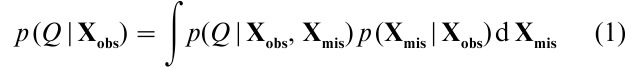
Equation (1) shows that the actual posterior density of Q can be obtained by averaging the complete-data posterior density over the posterior predictive distribution of X_mis. In principle, the set of multiple imputations under one model are repeated independent draws from p(X_mis |X_obs). Thus, multiple imputation allows the data analyst to approximate Eqn. (1) by separately analyzing each data set completed by imputation and then combining the results of the separate analyses.

2. Analyzing A Multiply-Imputed Data Set

The exact computation of the posterior distribution (Eqn. (1)) by simulation would require that an infinite number of values of X_mis be drawn from p(X_mis|X_obs). Fortunately, simple approximations work very well in most practical situations with only three to five imputations.

2.1 Inferences For Scalar Q

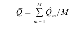
Suppose, as is typically true in the social and behavioral sciences, that if the data were complete, inferences for Q would be based on a point estimate Q, an associated variance/covariance estimate U, and a normal reference distribution. When data are missing and there are M sets of imputations for the missing data, the result is M sets of complete-data statistics, say, Q_m and U_m, m = 1,…, M.

The following procedure is useful for drawing inferences about Q from the multiply imputed data (Rubin 1987, Rubin and Schenker 1986). The point estimate of Q is the average of the M completed-data estimates,

and the associated variance estimate is

where U = ∑^M_m=1U_m/M is the average within-imputation variance, and B = ∑^M_m=1 (Q_m – Q)² /(M – 1) is the between-imputation variance (cf. the usual analysis of variance breakdown in Linear Hypothesis). The approximate reference distribution for interval estimates and significance tests is a t distribution with degrees of freedom

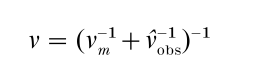
where ν_m = (M 1)γ⁻², ν_obs = ν_com(1 – γ)(ν­ + 1)/(ν_com + 3), γ = (1 + M^-1)B/T is the approximate Bayesian fraction of missing information, and ν_com is the complete-data degrees of freedom (see Barnard and Rubin 1999 for the derivation).

2.2 Significance Tests For Multicomponent Estimands

Multivariate analogues of the expressions given in the previous section for scalar Q are summarized by Rubin (1987, Sect. 3.4). Methods also exist for likelihood-ratio testing when the available information consists of point estimates and evaluations of the complete data log-likelihood-ratio statistic as a function of these estimates and the completed data.

With large data sets and large models, such as in the common situation of a multi-way contingency table, the complete-data analysis might produce only a test statistic and no estimates (cf. Multivariate Analysis: Discrete Variables (Overview)). Rubin (1987, Sect. 3.5) provided initial methods for situations with such limited information, and improved methods exist that require only the M complete-data χ² statistics (or equivalently the M complete-data P-values). These methods, however, are less accurate than methods that use the completed-data estimates.

3. Creating Multiple Imputations

Ideally, multiple imputations are M independent random draws from the posterior predictive distribution of X_mis under appropriate Bayesian modeling assumptions. Such imputations are called repeated imputations by Rubin (1987, Chap. 3). In practice, approximations often are used and work well.

3.1 Modeling Issues

An initial modeling issue in creating imputations is that the predictive distribution for the missing values should be conditional on all observed values. This consideration is particularly important in the context of a public-use database. Leaving a variable out of the imputation model is equivalent to assuming that the variable is not associated with the variables being imputed, conditionally given all other variables in the model; imputing under this assumption can result in biases in subsequent analyses, with estimated parameters representing conditional association pulled toward zero. Because it is not known which analyses will be carried out by subsequent users of a public-use database, ideally it is best not to leave any variables out of the imputation model. Thus, it is desirable to condition imputations on as many variables as possible and to use subject-matter knowledge to help select those variables that are likely to be used together in subsequent complete-data analyses, as by Clogg et al. (1991).

Imputation procedures can be based on explicit models or implicit models, or even combinations (see, e.g., Rubin 1987, Chap. 5, Rubin and Schenker 1991). An example of a procedure based on an explicit model is stochastic normal regression imputation, where imputations for missing values are created by adding normally distributed errors to predicted values obtained from a least-squares regression fit. A common procedure based on implicit models is hot-deck imputation, which replaces the missing values for an incomplete case by the values from a matching complete case, where the matching is carried out with respect to variables that are observed for both the incomplete case and complete cases.

The model underlying an imputation procedure, whether explicit or implicit, can be based on the assumption that the reasons for missing data are either ignorable or nonignorable (see Rubin 1976, and Statistical Data, Missing). The distinction between an ignorable and a nonignorable model can be illustrated by a simple example with two variables, X and Y, where X is observed for all cases whereas Y is sometimes missing. Ignorable models assert that a case with Y missing is only randomly different from a complete case having the same value of X. Nonignorable models assert that there are systematic differences between an incomplete case and a complete case even if they have identical X-values. An important issue with nonignorable models is that, because the missing values cannot be observed, there is no direct evidence in the data to address the assumption of nonignorability. It can be important, therefore, to consider several alternative models and to explore sensitivity of resulting inferences to the choice of model. In current practice, almost all imputation models are ignorable; limited experience suggests that in major surveys with limited amounts of missing data and careful design, ignorable models are satisfactory for most analyses (see, e.g., Rubin et al. 1995).

3.2 Incorporating Proper Variability

Multiple imputation procedures that incorporate appropriate variability across the M sets of imputations within a model are called ‘proper’ by Rubin (1987, Chap. 4) where precise conditions for a method to be proper are also given; also see Meng (1994) and Rubin (1996). Because, by definition, proper methods reflect sampling variability correctly, inferences based on the multiply-imputed data are valid from the standard repeated-sampling (i.e., design-based) frequentist perspective.

One important principle related to incorporating appropriate variability is that imputations should be random draws rather than best predictions. Imputing best predictions can lead to distorted estimates of quantities that are not linear in the data, such as measures of variability and correlation, and it generally results in severe underestimation of uncertainty and therefore invalid inferences.

For imputations to be proper, the variability due to estimating the model must be reflected along with the variability of data values given the estimated model. For this purpose, a two-stage procedure is often useful. Fixing parameters at a point estimate (e.g., the maximum likelihood estimate), across the M imputations and drawing X_mis from this distribution-generally leads to inferences based on the multiply-imputed data that are too sharp. First drawing the parameters from their joint posterior distributions is preferable.

The two-stage paradigm can be followed in the context of nonparametric methods such as hot-deck imputation as well as in the context of parametric models with formal posterior distributions for parameters. The simple hot-deck procedure that randomly draws imputations for incomplete cases from matching complete cases is not proper because it ignores the sampling variability due to the fact that the population distribution of complete cases is not known but rather is estimated from the complete cases in the sample. Rubin and Schenker (1986, 1991) discussed the use of the bootstrap to make the hot-deck procedure proper, and called the resulting procedure the ‘approximate Bayesian bootstrap.’ The two-stage procedure first draws a bootstrap sample from the complete cases and then draws imputations randomly from the bootstrap sample. Thus, the bootstrap sampling from the complete cases before drawing imputations is a nonparametric analogue of drawing values of the parameters of the imputation model from their posterior distribution before imputing conditionally upon the drawn parameter values. Heitjan and Little (1991) illustrated the use of bootstrap sampling to create proper imputations with a parametric model.

3.3 Choice Of M

The choice of M involves a tradeoff between simulating more accurately the posterior distribution and using a smaller amount of computing and storage. The effect of the value of M on accuracy depends on the fraction of information about the estimand Q that is missing (Rubin 1987, Chaps. 3, 4). With ignorable missing data and just one variable, the fraction of missing information is simply the fraction of data values that are missing. When there are several variables and ignorable missing data, the fraction of missing information is often smaller than the fraction of cases that are incomplete because of the ability to predict missing values from observed values; this is often not true with nonignorable missing data, however.

For the moderate fractions of missing information ( < 30 percent) that occur with most analyses of data from most large surveys, Rubin (1987, Chap. 4) showed that a small number of imputations (say, M = 3 or 4) results in nearly fully efficient estimates of Q. In addition, if proper multiple imputations are created, then a substantial body of work suggests that the resulting inferences generally have close to their nominal coverages or significance levels, even when the number of imputations is moderate (Clogg et al. 1991, Heitjan and Little 1991, Rubin and Schenker 1986 and additional publications cited by Rubin 1996).

3.4 Use Of Iterative Simulation Techniques

Recent developments in iterative simulation, such as data augmentation (Tanner and Wong 1987) and Gibbs sampling (Gelfand and Smith 1990), can facilitate the creation of multiple imputations in complicated parametric models. Consider a joint model for X_obs and X_mis governed by a parameter, say θ. The data augmentation (Gibbs sampling) procedure that results in draws from the posterior distribution of θ produces multiple imputations as well. (Schafer 1997) developed algorithms that use iterative simulation techniques to multiply impute data when there are arbitrary patterns of missing data and the missing-data mechanism is ignorable.

4. Some Recent Applications Of Multiple Imputation In Social-Science Research

To illustrate settings in which multiple imputation can be useful, brief descriptions of several recent applications of multiple imputation to social-science research are now given. References to many other examples are provided by Rubin (1996).

4.1 Multiple Imputation To Achieve Comparability Of Industry And Occupation Codes Over Time

The first large-scale application of multiple imputation for public-use data involved employment information from the decennial census. In each census, such information is obtained from individuals in the form of open-ended descriptions of occupations. These descriptions are then coded into hundreds of industries and occupations, using procedures devised by the Census Bureau. Major changes in the procedures for the 1980 census resulted in public-use databases from the 1980 census with industry and occupation codes that were not directly comparable to those on publicuse databases from previous censuses, in particular, the 1970 census. This lack of comparability made it difficult to study such topics as occupation mobility and labor force shifts by demographic characteristics.

Because of the size of the 1970 public-use databases (about 1.6 million cases) and the inaccessibility of the original descriptions of occupations, which were stored away on microfilm, it would have been prohibitively expensive to recode the 1970 data according to the 1980 scheme. There existed, however, a smaller (about 127,000 cases) double-coded sample from the 1970 census, that is, a sample with both 1980 and 1970 occupation codes, that had been created for other purposes. Based on Bayesian models estimated from the double-coded sample, five sets of 1980 codes were imputed for the 1970 public-use database as outlined by Clogg et al. (1991). Simulations described by Rubin and Schenker (1987) support the validity of multiple-imputation inferences in this application. Finally, analyses described by Schenker et al. (1993) demonstrated potential gains in efficiency from basing analyses on the multiply imputed public-use sample rather than on the smaller double-coded sample, even though the actual 1980 codes are known on the latter and unknown on the former.

4.2 Multiple Imputation For Missing Data In A National Health Survey

The National Health and Nutrition Examination Survey (NHANES) is conducted by the National Center for Health Statistics (NCHS) to assess the health and nutritional status of the United States population and important subgroups. The data from NHANES are obtained through household interviews and through standardized physical examinations. NCHS has recently made available a database from the third NHANES, in which multiple imputation based on complicated multivariate models and iterative simulation techniques was used to handle missing data. This multiple-imputation project is significant because it demonstrates the feasibility of generating proper multiple imputations for a public-use sample obtained by a complex survey design with many observations and variables, varying rates of missingness on key variables of interest, and various patterns of nonresponse.

Documentation available with the database contains descriptions of the models and procedures used to multiply impute data for the third NHANES, as well as descriptions and examples of how to analyze the multiply-imputed data. Earlier work on the project is summarized by Schafer et al. (1996). In particular, a simulation study of the validity of multiple-imputation interval estimates was conducted based on a hypothetical population constructed from data from the third NHANES as well as earlier versions of NHANES. Results indicated that the imputation procedures were successful in creating valid design-based repeated-sampling inferences.

4.3 Multiple Imputation In A Study Of Drinking Behavior With Follow-Up For Nonresponse

The Normative Aging Study was a longitudinal study of community-dwelling men conducted by the Veterans Administration in Boston. In a survey on drinking behavior conducted as part of this study, a large fraction of the men surveyed provided essentially complete information, whereas for a smaller fraction, there was background information available but no information on drinking behavior. Because drinking behavior is a sensitive subject, there was concern that such nonresponse might be nonignorable.

In a follow-up survey, information on drinking behavior was obtained from about one-third of the initial nonrespondents. Glynn et al. (1993) multiply imputed data on drinking for the roughly two-thirds of the initial nonrespondents who remained, under the assumption that, in the stratum of initial nonrespondents, given the follow-up information as well as the background information that had been collected previously, nonresponse was now ignorable. It was found that inferences about the effect of retirement status on drinking behavior (adjusting for age) were very sensitive to whether the multiply-imputed data or only the data for the initial respondents were used.

4.4 A Contest: Multiply Imputing The Consumer Expenditure Survey

Raghunathan and Rubin (1997) describe a simulation study to examine the frequentist properties of various methods of generating multiple imputations that was funded by the United States Bureau of Labor Statistics (BLS). The simulation study used real data from the Consumer Expenditure Survey (CES), which is the most detailed source of expenditures, income, and demographics collected by the US government. The objective of the simulation study was to compare frequentist performance of imputation-generation methods that differed by whether they fully accounted for parameter uncertainty and/or whether they conditioned on all observed variables. The recommended approach in the multiple-imputation literature is to generate imputations that account for all sources of uncertainty and condition on all observed information. Some BLS staff questioned this recommendation, preferring to use simpler methods for generating imputations that do not account for parameter uncertainty and exclude some variables, in this case measures of expenditure, because of concerns about endogeneity.

The artificial population from which the simulation samples were drawn consisted of complete reporters from the CES. BLS staff generated 200 independent samples, each of approximate size 500 from the constructed population, then imposed an ignorable monotone missing-data mechanism on each sample, resulting in 200 incomplete samples. Two variables in the samples had missing data: ethnicity and income. The incomplete samples were then sent to the multiple-imputation team, who were unaware of the exact nature of the missing-data mechanism, for analysis. All the variables used in the missing-data mechanism as well as some other variables were provided to the multiple-imputation team without noting which were which.

The multiple-imputation team generated five imputations for each incomplete sample under a variety of approaches: accounting for parameter uncertainty and using all variables, accounting for parameter uncertainty but excluding some variables (expenditure information), ignoring parameter uncertainty and using all variables, and ignoring parameter uncertainty and excluding some variables. The multiply-imputed samples were sent to BLS for analysis. The results were that the recommended method for generating imputations, accounting for parameter uncertainty and including all variables, produced confidence intervals that had the nominal coverage whereas all of the other methods produced intervals that undercovered, with the method that ignored parameter uncertainty and excluded expenditure information having the worst performance.

4.5 Multiple Imputation In The Survey Of Consumer Finances

Kennickell (1998) reported on the use of multiple imputation for handling missing data and for disclosure limitation in the Survey of Consumer Finances (SCF). The SCF is a triennial survey conducted by the US Board of Governors of the Federal Reserve System in cooperation with the Statistics of Income Division of the Internal Revenue Service. The SCF is a major source of detailed asset, liability, and general financial information and includes over 2,700 questions. The SCF is focused on the details of households’ finances, and due to the sensitivity of this topic it suffers from substantial unit and item nonresponse rates. In addition, because the SCF asks many questions about monetary amounts, the skip patterns in the SCF are very complex, resulting in complicated response pat terns. These factors make direct analysis of the incomplete SCF data extremely difficult for general users.

To combat the problem of missing data in the SCF, multiply-imputed versions of the SCF have been and continue to be released to the public. The SCF multiple imputations were generated using a novel variation of the Gibbs sampling algorithm that combines great modeling flexibility with computational tractability. Multiple imputation is also being used for disclosure limitation of income information in the SCF Kennickell (1997), based on ideas put forth by Rubin (1993) for protecting sensitive data by creating via imputation completely artificial populations.

4.6 Handling ‘Don’t Know’ Survey Responses In The Slovenian Plebiscite

The Republic of Slovenia separated from Yugoslavia on October 8, 1991. One year before, Slovenians voted on independence through a plebiscite. Of eligible voters, 88.5 percent voted in favor of independence. To predict the results of the plebiscite, the Slovenian government inserted questions into the Slovenian Public Opinion (SPO) Survey that was conducted four weeks prior to the plebiscite. The SPO is a face-to-face survey of approximately 2,000 voting-age Slovenians containing questions on many aspects of Slovenian life, including education and health. It has been conducted one to two times each year for the past 30 years. The plebiscite-related questions inserted into the SPO had three possible responses: ‘yes,’ ‘no,’ and ‘don’t know’(DK). In some surveys DK is a valid response, but in the plebiscite everyone votes either ‘yes’ or ‘no’ to the issue of independence, either by voting in person or by staying home (effectively a ‘no’ vote). Hence, the DK responses to the SPO survey question can be viewed as missing or masked data, masking either a ‘yes’ or ‘no’ plebiscite response.

Rubin et al. (1995) analyzed the SPO results with the goal of predicting the true percentage of voters in favor of independence. They treated the DK responses as missing data and considered ignorable and nonignorable missing-data mechanisms. Their prediction from a straightforward ignorable model was very accurate, while that from their most realistic nonignorable model was substantially far from the truth. The results are particularly interesting because the predictions were obtained before the true percentage was known and indicate that simple ignorable models can produce better answers than more complex and seemingly more plausible nonignorable models.

5. Conclusion

Multiple imputation is a general approach for handling the pervasive and often challenging problem of reaching statistically valid inferences from incomplete data. It was derived from a Bayesian perspective but produces inference procedures that have excellent frequentist properties. Generating multiple imputations can be difficult, and fortunately computer software is appearing that aids in this task (see below), but analyzing a multiply-imputed data set was designed to be almost as easy as analyzing a complete data set. A multiple-imputation inference is obtained by applying a complete-data inference procedure to each of the multiple data sets completed by imputation and then combining these estimates using simple combining rules. To learn more about multiple imputation (see Rubin 1987, 1996 and Schafer 1997).

There is currently only a limited amount of software for generating multiple imputations under multivariate complete-data models and for analyzing multiply-imputed data sets (i.e., completing the data sets, running the complete-data analyses, and combining the complete-data outputs), but the situation appears to be rapidly improving. For generating imputations, software to implement the methodology developed by Schafer (1997) has been written for the S-PLUS (Mathsoft 2001) statistical package and is freely available on the Internet. This software includes programs for multiple imputation in the contexts of incomplete multivariate normal data, incomplete categorical data, and incomplete data under the general location model allowing both categorical and multivariate normal variables.

A revised and expanded version of this software, including facilities for easily analyzing multiply-imputed data, has been incorporated into recent release of S-PLUS. SOLAS (Statistical Solutions 2000), the first commercial product for multiple imputation, combines a graphical user interface and integrated environment for analyzing multiply-imputed data with flexible and efficient methods of generating imputations that exploit the computational and modeling advantages of near monotone missing-data patterns. SAS Institute is developing procedures for analyzing and generating multiply imputed data under a variety of parametric models. These procedures are expected to be available in the very near future. The web site www.multiple-imputation.com contains a fairly complete list of software for multiple imputation and serves as source for news and events associated with multiple imputation.

Bibliography:

1. Barnard J, Rubin D B 1999 Small-sample degrees of freedom with multiple imputation. Biometrika 86: 948–55
2. Clogg C C, Rubin D B, Schenker N, Schultz B, Weidman L 1991 Multiple imputation of industry and occupation codes in census public-use samples using Bayesian logistic regression. Journal of the American Statistical Association 86: 68–78
3. Gelfand A E, Smith A F M 1990 Sampling-based approaches to calculating marginal densities. Journal of the American Statistical Association 85: 398–409
4. Glynn R J, Laird N M, Rubin D B 1993 Multiple imputation in mixture models for nonignorable nonresponse with follow-ups. Journal of the American Statistical Association 88: 984–93
5. Heitjan D F, Little R J A 1991 Multiple imputation for the fatal accident reporting system. Applied Statistics 40: 13–29
6. Kennickell A B 1997 Multiple imputation and disclosure protection: The case of the 1995 Survey of Consumer Finances. In: Record Linkage—1997: Proceedings of an International Workshop and Exposition. US Office of Management and Budget, Washington, DC, pp. 248–67
7. Kennickell A B 1998 Multiple imputation in the Survey of Consumer Finances. In: ASA Proceedings of the Business and Economic Statistics Section. American Statistical Association, Alexandria, VA, pp. 11–20
8. Mathsoft 2001 S-PLUS User’s Manual, Version 6. StatSci, a division of Mathsoft Inc., Seattle, WA
9. Meng X-L 1994 Multiple-imputation inferences with uncongenial sources of input (Disc: P558–573). Statistical Science 9: 538–58
10. Raghunathan T E, Rubin D B 1997 Roles for Bayesian techniques in survey sampling. In: Proceedings of the Survey Methods Section of the Statistical Society of Canada. Statistical Society of Canada, McGill University, Montreal, PQ, pp. 51–5
11. Rubin D B 1976 Inference and missing data. Biometrika 63: 581–90
12. Rubin D B 1987 Multiple Imputation for Nonresponse in Surveys. Wiley, New York
13. Rubin D B 1993 Comment on ‘Statistical Disclosure Limitation’. Journal of Official Statistics 9: 461–8
14. Rubin D B 1996 Multiple imputation after 18 + years (Pkg: P473–520). Journal of the American Statistical Association 91: 473–89
15. Rubin D B, Schenker N 1986 Multiple imputation for interval estimation from simple random samples with ignorable nonresponse. Journal of the American Statistical Association 81: 366–74
16. Rubin D B, Schenker N 1987 Interval estimation from multiply-imputed data: A case study using census agriculture industry codes. Journal of Official Statistics 3: 375–87
17. Rubin D B, Schenker N 1991 Multiple imputation in health-care databases: An overview and some applications. Statistics in Medicine 10: 585–98
18. Rubin D B, Stern H S, Vehovar V 1995 Handling ‘Don’t know’ survey responses: The case of the Slovenian Plebiscite. Journal of the American Statistical Association 90: 822–8
19. Schafer J L 1997 Analysis of Incomplete Multivariate Data. Chapman and Hall, New York
20. Schafer J L, Ezzati-Rice T M, Johnson W, Khare M, Little R J A, Rubin D B 1996 The NHANES III multiple imputation project. In: ASA Proceedings of the Section on Survey Research Methods. American Statistical Association, Alexandria, VA, pp. 28–37
21. Schenker N, Treiman D J, Weidman L 1993 Analyses of public use Decennial Census data with multiply imputed industry and occupation codes. Applied Statistics—Journal of the Royal Statistical Society Series C 42: 545–56
22. Statistical Solutions 2000 SOLAS for Missing Data Analysis 2.0. Statistical Solution Ltd., Cork, Ireland
23. Tanner M A, Wong W H 1987 The calculation of posterior distributions by data augmentation. Journal of the American Statistical Association 82: 528–40