Multivariate Approaches to Exploratory Data Analysis Research Paper

1. The Curse Of Dimensionality

The Curse of Dimensionality (COD) was coined by the mathematician Richard Bellman in the context of approximation theory. For statisticians, the term has a slightly different connotation, and refers to the difficulty of finding predictive functions for the response variable Y using explanatory variables X p when p is large.

There are three nearly equivalent formulations of the COD, each of which offers a useful perspective on the problem:

(a) When p is large, nearly all datasets are sparse.

(b) The number of possible regression functions increases faster than exponentially in the dimension p of the space of explanatory variables.

(c) When p is large, nearly all datasets show multicollinearity (and its nonparametric generalization, concurvity).

These problems can be reduced if data are collected using a careful statistical design, such as Latin hyper-cube sampling. However, except in simulation experiments, this is difficult to do.

The first formulation is the most common. It refers to the fact that if one takes five random points in the unit interval, they tend to be close neighbors, while five points in the unit square and the unit cube are increasingly separated. Thus as dimension increases, a fixed sample size provides less local information. One way to quantify this is to ask what is the side-length of a p-dimensional cube that is expected to contain half of the data that are randomly (un iformly) distributed in the unit cube? The answer is (.5)^1/p, and this increases towards 1 as p gets large. Thus, the expected number of observations in a fixed region of R^p goes to zero, implying little information in the data about the local relationship between Y and X. Therefore, one requires very large sample sizes before nonparametric regression is feasible in higher dimensions.

The second formulation of the COD has an information-theoretic quality. There are many possible models one can fit when p is large, and it is difficult for a finite sample to successfully discriminate among those alternatives in selecting and fitting the best model. To see this, suppose one considers only polynomial models of degree 2 or less. For p=1 there is a single explanatory variable, and the seven possible models are:

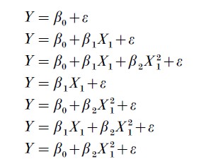
where ε denotes random noise in the measurement of Y. When p=2, there are 63 possible models (including terms of the form X₁ X₂ ), and a simple comb inatorvia l argument shows that, in general, there are 2^1+p+p(p+1)/2 polynomial models of degree 2 or less. Since realistic applications typically need to explore much more complicated functional relationships than just low degree polynomials, one needs vast amounts of data to distinguish among so many possibilities.

The third formulation is more subtle. In traditional multiple regression, multicollinearity occurs when two or more explanatory variables are correlated, so that the data mostly lie in an affine subspace of p (e.g., close to a line or a plane within a volume). When this happens, there are an infinite number of models that fit the data almost equally well, but these models can be very different with respect to predictions of future values that do not lie in the subspace. As p increases, the number of possible subspaces gets large very rapidly, and thus, just by chance, any realistically finite dataset will tend to concentrate along a few of them. The problem is aggravated in nonparametric regression—the analogue of multicollinearity occurs when data concentrate along a smooth manifold within R^p, and there are many more smooth manifolds than affine subspaces.

The COD poses both practical and theoretical difficulties for researchers who want to let the data select an adequate model. These problems have been deliberately addressed in a body of statistical literature that began in the mid-1980s, and the remainder of this research paper sketches the kinds of partial solutions that have been obtained. Further discussion of the COD and its consequences for regression may be found in Hastie and Tibshirani (1990) and Scott and Wand (1991).

2. Methods Of Nonparametric Regression

Among the many new methods in nonparametric regression, we focus on six that have become widely used. These are the additive model (AM), alternating conditional expectation (ACE), projection pursuit regression (PPR), recursive partitioning regression (RPR), multivariate adaptive regression splines (MARS), and locally weighted regression (LOESS).

2.1 The Additive Model (AM)

The AM has been developed by several authors; Buja et al. (1989) describe the background and early development. The simplest AM has the form

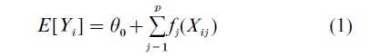
where the functions f_j are unknown (but have mean zero).

Since the f_j are estimated from the data, the AM avoids the traditional assumption of linearity in the explanatory variables; however, it retains the assumption that explanatory variable effects are additive. Thus, the response is modeled as the sum of arbitrary smooth univariate functions of the explanatory variables, but not as the sum of multivariate functions of the explanatory variables. One needs a reasonably large sample size to estimate each f_j, but under the model posted in (Eqn. 1), the sample size requirement grows only linearly in p.

The backfitting algorithm is the key procedure used to fit an additive model; operationally, the algorithm proceeds as follows:

(a) At the initialization step, define functions f_j⁽⁰⁾≡ 0; also, set θ₀=Y.

(b) At the ith iteration, estimate f_i^(t+1) by

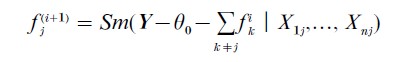
for j=1,…, p.

(c) Check whether |f_j^(t+1)-f_j^(t)|<δ for all j=1,…, p, where δ is the convergence tolerance. If not, return to step 2; otherwise, use the f_j⁽ⁱ⁾ as the additive functions f_j in the model.

This algorithm requires a smoothing operation (such as kernel smoothing or nearest-neighbor averaging) indicated by Sm(·|·). For large classes of smoothing functions, the backfitting algorithm converges to a unique solution.

One can slightly generalize the AM by allowing it to sum functions that involve a small number of prespecified explanatory variables. For example, if one felt that income prediction in the AM would be improved by adding a bivariate function that depended on both a person’s IQ and their years of education, then a bivariate smoother could be used to fit such a term in the second step of the backfitting algorithm.

2.2 Alternating Conditional Expectations (ACE)

An extension of the AM permits transformation of the response variable as well as of the p explanatory variables. This depends on the ACE algorithm, developed by Breiman and Friedman (1985), which fits the model

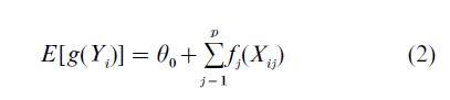
where all conditions are as given for (Eqn. 1), except g is an unspecified function, scaled to satisfy the technically necessary constraint that var[ g(Y )]=1 (otherwise, the zero transformation would be trivially perfect).

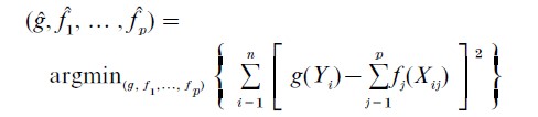
Given variables Y_i and X_i, one wants g, θ₀ , and f₁,…, f_p so that E[g(Y_i)|X_i]-θ₀-∑^p_j=1f_j(X_ij) is independent error. Formally, one solves

where g satisfies the unit variance constraint. Operationally, one proceeds as follows:

(a) Estimate g by g⁽⁰⁾ , obtained by applying a smoother to the Y_i values and standardizing the variance. Set f_j⁽⁰⁾ ≡ 1 for all j =1,…, p.

(b) Conditional on g^(k−1) (Y_i), apply the backfitting algorithm to estimate f₁^{( k)} ,…, f_p ^(k).

(c) Conditional on the sum of f₁^(k),…, f^(k)_p, obtain g^(k) by applying the backfitting algorithm (this interchanges the role of the explanatory and response variables). Standardize the new function to have unit variance.

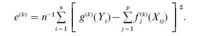
(d) Test for convergence: is |e^(k)-e^{(k− 1)} |≤ δ, where δ is a prespecified small value and

If convergence is sufficient, set g=g^(k), f_j =f_j^(k); otherwise go to step 2.

Steps 2 and 3 calculate smoothed expectations, each conditional upon functions of either the response or the explanatory variables; this alternation gives the method its name.

The ACE analysis finds sets of functions for which the linear correlation of the transformed response variable and the sum of the transformed explanatory variables is maximized. Thus ACE is more closely related to correlation analysis and the multiple correlation coefficient than to regression. Since ACE does not aim directly at regression, it has some undesirable features, for example, it treats the response and explanatory variables symmetrically, small changes can lead to radically different solutions (cf. Buja and Kass 1985), and it does not reproduce model trans- formations.

To overcome some of these drawbacks in ACE, Tibshirani (1988) invented a variation called AVAS which imposes a variance-stabilizing transformation in the ACE backfitting loop for the explanatory variables. The basis for this modification is technical, but it improves the theoretical properties of ACE for regression applications.

2.3 Projection Pursuit Regression (PPR)

The AM considers sums of functions taking arguments in the natural coordinates of the space of explanatory variables. When the underlying function is additive with respect to variables formed by linear combinations of the original explanatory variables, the AM is inappropriate. PPR was designed by Friedman and Stuetzle (1981) to handle such cases.

Heuristically, suppose there are only two explanatory variables and that the regression surface looks like a piece of corrugated aluminum. If that surface is oriented so that the corrugations are parallel to one of the axes of the explanatory variables (and hence perpendicular to the other axis), then the AM is an excellent technique. But if the aluminum surface is turned so that the corrugations are not parallel to a natural axis, the AM will fail but PPR would work.

PPR employs the backfitting algorithm and a conventional numerical search routine, such as Gauss–Newton, to fit a model of the form

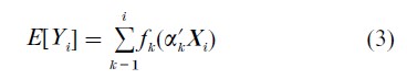
where the α₁ ,…, α_r determine a set of r linear combinations of the explanatory variables. These linear combinations are analogous to those used in principal components analysis (cf. Flury 1988). An important difference is that these vectors need not be orthogonal, but are chosen to maximize the predictive accuracy of the model as assessed through cross-validation.

Specifically, PPR alternately calls two routines. The first conditions upon a set of pseudo variables that are linear combinations of the original variables; these are used in the backfitting algorithm to find an AM that sums functions whose arguments are the pseudo variables (which need not be orthogonal). The second routine conditions upon the estimated AM functions, and then searches for linear combinations of the original variables that maximize the fit. Alternating iterative application of these methods converges, very generally, to a unique solution.

PPR can be hard to interpret when r>1 in (Eqn. 3). If r is allowed to grow without bound, PPR is consistent, in the sense that as the sample size increases, the fitted regression function will converge to the true regression function.

Unlike the AM, PPR is invariant to affine transformations of the data; this is appealing when the variables used in the research are measured in the same units and have similar scientific rationales. For example, PPR might sensibly be used in biometry to predict a person’s weight when the measurements are different long-bone lengths, but it would be less advisable to use PPR when one explanatory variable is ulna length and another is the thickness of the layer of subcutaneous fat.

PPR is very similar to neural net methods. The primary difference is that neural net techniques usually assume that the functions f_k are sigmoidal, whereas PPR allows more flexibility. Zhao and Atkeson (1992) show that PPR has similar asymptotic properties to standard neural net techniques.

2.4 Recursive Partitioning Regression (RPR)

RPR methods have become popular since the advent of CART (Classification and Regression Tree) methodology, developed by Breiman et al. (1984). This research paper is not concerned with classification problems, and so the basic RPR algorithm we consider fits a model of the form

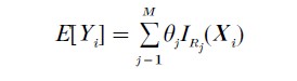
where the R₁,…, R_M are rectangular regions that partition R^p, and I_Rj (X_i) is an indicator function taking the value 1 if and only if X_iϵR_j, and otherwise is zero. Here θ_j is the estimated value for all responses whose explanatory variables lie in R_j.

RPR is designed to be very good at finding local low-dimensional structure in functions that have high- dimensional global dependence. It is consistent; also, it has a powerful graphic representation as a decision tree, which increases interpretability. However, many elementary functions are awkward for RPR, for example, it would approximate a simple linear regression by a stairstep function. In higher dimensions it is usually difficult to discover when the fitted piecewise constant model approximates a standard smooth function.

To be concrete, suppose one were trying to use RPR to predict income from gender and years of education. The algorithm would search all possible intermediate splits in the training sample observations for both explanatory variables, and perhaps decide that the most useful first split is at 12.5 years. For training sample cases with more than high school education, the algorithm repeats the search and perhaps finds the next useful split is at 16.5 years, corresponding to college graduation. Similarly, for those with no education beyond high school, the algorithm searches the cases and may decide to split on gender. This search process repeats in each subset of the training data formed by previous divisions, and eventually no potential split achieves sufficient reduction in variance to justify further partitioning. At that point RPR fits the average of all the cases within the most refined subsets as the predictions θ_j, and represents the sequence of splits in a decision tree. (Note: Some RPR algorithms are more complex, for example, CART will ‘prune back’ the final tree, removing splits better balance fit in the training sample against predictive error.)

2.5 Multivariate Adaptive Regression Splines (Mars)

Friedman (1991) describes a method that combines PPR with RPR, using multivariate adaptive regression splines. This procedure fits a model that is the weighted sum of multivariate spline basis functions (tensorspline basis functions), and takes the form

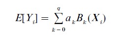
where the coefficients a_k are determined in the course of (generalized) cross-validation fitting. The constant term follows by setting B₀(X₁,…, X_n) ≡1, and the other multivariate splines are products of univariate spline basis functions

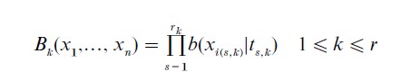
Here the subscript i(s, k) indicates a particular explanatory variable, and the basis spline in that variable has a knot at t_s,k. The values of q, the r₁,…, r_q, the knot sets, and the appropriate explanatory variables for inclusion are all determined adaptively from the data.

MARS admits a decomposition similar to that obtained from an analysis of variance; it can be represented in a table and similarly interpreted. MARS is designed to perform well whenever the true function has low local dimension. The procedure automatically accommodates interactions between variables and variable selection.

2.6 Locally Weighted Regression (LOESS)

Cleveland (1979) proposed a locally weighted regression technique. Rather then simply taking a local average, LOESS fits a model of the form E[Y ]=θ(x)`x where

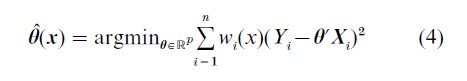
and w_i is a weighting function that controls the influence of the ith observation according to the distance and direction of X_i from x.

LOESS has good consistency properties, but can be inefficient at discovering some relatively simple structures in data. Although not originally designed for high-dimensional regression, its use of local information makes it quite flexible. Cleveland and Devlin (1988) have generalized LOESS to use polynomial regression instead of the linear regression θ`X_i in (Eqn. 4), but that does not usually have a strong impact on performance.

3. Comparisons

Currently, our understanding of comparative nonparametric regression performance consists of a scattering of theoretical and simulation results. The key sources of information are:

(a) Donoho and Johnstone (1 989) make asymptotic comparisons in terms of the L² norm criterion

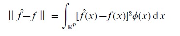
where p is the dimension of the space and φ is the density of the standard normal distribution (i.e., they use a weighted mean integrated squared error (MISE) criterion). They find that projection-based regression methods (PPR, MARS) perform significantly better for radial functions, whereas kernel-based regression (LOESS) is superior for harmonic functions. Radial functions are constant on hyperspheres centered at 0, whereas harmonic functions vary periodically on such hyperspheres—a ripple in a pond is radial; an Elizabethan ruff is harmonic.

(b) Friedman (1991) reports simulation studies of MARS alone, and related work is described by his discussants. Friedman examines several criteria; the main ones are scaled versions of MISE and predictive squared error (PSE), and a criterion based on the ratio of a generalized cross-validation error estimate to PSE. From our standpoint, the most useful conclusions are that:

(i) When the data are pure noise in five and 10 dimensions, for sample sizes of 50, 100, and 200, MARS and AM are roughly comparable and unlikely to find spurious structure.

(ii) When the data are generated from the additive function of five variables

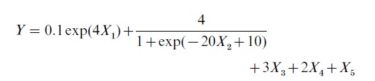
with five additional noise variables and sample sizes of 50, 100, and 200, MARS had a slight but clear tendency to overfit, especially at the smallest sample sizes.

All of Friedman’s simulations, except the pure noise condition, have high signal-to-noise ratios.

 (c) Tibshirani (1988) gives theoretical reasons why AVAS has superior properties to ACE (but notes that consistency and behavior under model misspecification are open questions). He describes a simulation experiment that compares ACE to AVAS in terms of weighted MISE on samples of size 100, finding that AVAS and ACE are similar, but that AVAS performs better than ACE when correlation is low.

(d) Barron (1991, 1993) shows that in a somewhat narrow sense, the mean integrated squared error of neural net estimates for a certain class of functions has order O(1/m)+O(mp /n)ln n, where m is the number of nodes, p is the dimension, and n is the sample size. This is linear in the dimension, evading the COD; similar results were subsequently obtained by Zhao and Atkeson (1992) for PPR, and it is likely that the result holds for MARS, too. These results may be less applicable than they seem; Barron’s class of functions are those whose Fourier transform g satisfies J| w | | g(w) | dw<c for some fixed c, and this excludes such standard cases as hyperflats, and becomes smoother as dimension increases.

(e) De Veaux et al. (1993) compared MARS and a neural net on two functions, finding that MARS was faster and more accurate in terms of MISE.

The broad conclusions include (a) model parsimony is increasingly valuable in high dimensions; (b) hierarchical models based on sums of piecewise-linear terms are relatively good; and (c) for any method one can find datasets on which it excels and datasets on which it fails badly.

These short, often asymptotic, explorations do not provide sufficient understanding for users to make an informed choice among regression techniques. Instead, a practitioner might hold out a portion of the data, apply many regression techniques to the rest of the data, and use the models that are built to predict the hold-out sample. Whichever method achieves minimum prediction error is probably the most appropriate for that application.

Bibliography:

1. Barron A R 1991 Complexity regularization with applications to artificial neural networks. In: Roussas G (ed.) Nonparametric Functional Estimation. Kluwer, Dordrecht, The Netherlands, pp. 561–76
2. Barron A R 1993 Universal approximation bounds for superpositions of a sigmoidal function. IEEE Transactions on Information Theory 39: 930–45
3. Breiman L, Friedman J H 1985 Estimating optimal transformations for multiple regression and correlation. Journal of the American Statistical Association 80: 580–98
4. Breiman L, Friedman J, Olshen R A, Stone C 1984 Classification and Regression Trees. Wadsworth, Belmont, CA
5. Buja A, Hastle T, Tibshirani R 1989 Linear smoothers and additive models. Annals of Statistics 17: 453–510
6. Buja A, Kass R 1985 Estimating optimal transformations for multiple regression and correlation. Journal of the American Statistical Association 80: 602–7
7. Cleveland W 1979 Robust locally weighted regression and smoothing scatter plots. Journal of the American Statistical Association 74: 829–36
8. Cleveland W, Devlin S 1988 Locally weighted regression: An approach to regression analysis by local fitting. Journal of the American Statistical Association 83: 596–610
9. De Veaux R D, Psichogios D C, Ungar L H 1993 A comparison of two nonparametric estimation schemes: MARS and neural networks. Computers in Chemical Engineering 17: 819–37
10. Donoho D L, Johnstone I M 1989 Projection-based approximation and a duality with kernel methods. Annals of Statistics 17: 58–106
11. Friedman J H 1991 Multivariate additive regression splines. Annals of Statistics 19: 1–66
12. Friedman J H, Stuetzle W 1981 Projection pursuit regression. Journal of the American Statistical Association 76: 817–23
13. Flury B 1988 Common Principal Components and Related Multivariate Models. Wiley, New York
14. Hastie T J, Tibshirani R J 1990 Generalized Additive Models. Chapman and Hall, London
15. Scott D W, Wand M P 1991 Feasibility of multivariate density estimates. Biometrika 78: 197–205
16. Tibshirani R 1988 Estimating transformations for regression via additivity and variance stabilization. Journal of the American Statistical Association 83: 394–405
17. Zhao Y, Atkeson C G 1992 Some approximation properties of projection pursuit networks. In: Moody J, Hanson S J, Lippmann R P (eds.) Advances in Neural Information Processing Systems 4. Morgan Kaufmann, San Matco, CA, pp. 936–43