Systems Modeling Research Paper

A number of fundamental characteristics of systemhood in the social and biological sciences will be discussed. These characteristics concern general types of relationships, in conformance with Klir’s (1991) definition. In contrast, specific relationships can be of any kind, like semantic relationships in cognitive systems, associative relationships in behavioral systems, synaptic relationships in neural systems, etc. From a general perspective, such specific relationships can each be conceived as a mapping in an abstract space, where this space is spanned up by generalized coordinates indexed by location and time. In this abstract setting, location-like relationships involve geometrical patterns and forms, timelike relationships involve dynamic regimes, and relationships involving both location and time pertain to spatiotemporal patterns. In this research paper, only timelike relationships can be considered in detail. However, much of the discussion generalizes rather straightforwardly to spatial and spatiotemporal aspects of systemhood.

Perhaps the most basic characteristic of systemhood is stability. Stability is a multifaceted characteristic. On the one hand, it pertains to the relationships of a system with its environment, how a system reacts to external inputs. This is the more classical variant of stability in which various types of equilibrium are distinguished, associated with distinct dynamic responses to environmental perturbations. On the other hand, stability characterizes the internal relationships between components of a system, how these relationships accommodate to endogenous changes. This more modern variant of stability concerns the changes in within-system types and number of equilibria under slow (so-called adiabatic) variation of system parameters. In between these classical and modern variants of stability we find equilibrium concepts associated with dynamic game theory.

In what follows the focus will be on a modern conceptualization of stability. That is, a consideration of qualitative changes in the equilibria of systems due to slow continuous variation of system parameters. Modern approaches to stability include much more than this; for instance, the recently discovered new equilibrium types (strange attractors associated with deterministic chaotic dynamic regimes). But attention will be restricted to qualitative changes in equilibria, because this has more definite implications for the social and behavioral sciences. A general theory of sudden qualitative changes, including methodological guidelines and some applications, will be outlined.

Another important characteristic of systemhood, closely related to stability, is homeostasis. The reason why it is considered separately is because in theoretical treatises the ubiquity of homeostatic processes in neurological and physiological systems is often emphasized, yet in actual empirical research it is equally often neglected. It will be shown, to the best of our knowledge for the first time in the social scientific literature, what are the expected consequences of homeostasis for empirical studies of, for instance, the biological bases of personality and behavior.

The final characteristic of systemhood to be considered is difficult to summarize with a single label. The characteristic concerned is related to the wellknown slogan: ‘The whole is more than its parts.’ This slogan could be elaborated as a new logic of part– whole relationships for general systems, but that is not our present endeavor. Yet the possibility of a whole transcending its constituent parts also bears on a number of fundamental issues such as unity, individuality, and other questions concerning the lack of comparability of systems that are composed of the same parts, but may differ at some higher level. In the closing sections it will be shown that taking the individuality of systems seriously leads to entirely new psychometric concepts and to a vindication of the so-called Developmental Systems paradigm.

1. Statistical Systems Modeling

To provide a proper setting for the discussion of characteristics of systemhood, a preliminary overview of statistical systems modeling will be given. For this purpose a canonical representation of systems, the socalled state–space model, is introduced. This canonical state–space model will only be used for the purpose of clarification. There exists an extensive literature on system identification, parameter estimation and hypothesis testing (cf. Elliott et al. 1995) which can be consulted for further details.

The state–space model concerned is defined as:

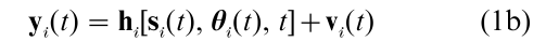
In Eqn. (1a) s_i(t) denotes the state of system i at time t, a vector-valued (hence bold-faced) latent (i.e., not directly observed) process. The difference equation (1a) expresses the dynamics of the state process of system i: s_i(t + 1) is related to s_i(t) by some function f_i, where fi also may depend on time t as well as on a vector-valued parameter θ_i(t). The latter parameter θ_i(t) itself may vary in time. The remaining term w_i(t + 1) in Eqn. (1a) denotes random variation in s_i(t + 1) which cannot be predicted on the basis of fi. In Eqn. (1b) y_i(t) denotes the observed (manifest) vector- valued process of system i at time t. The function hi expresses the dependence of y_i(t) on the state s_i(t), where hi also may depend on time t as well as on the parameter θ_i(t). The remaining term vi(t) in Eqn (1b) denotes random measurement error.

The state–space model Eqn. (1) is quite general, although an even more general definition could be given. But for our present purposes Eqn. (1) suffices. Through additional specifications, many well-known types of process models are obtained as special instances of Eqn. (1). These specifications mainly concern the measurement scales of the state process s_i(t) and manifest process y_i(t), which each can be metrical or categorical; the forms of fi and hi, which can be linear or nonlinear, and the distributional assumptions characterizing w_i(t) and vi(t). Furthermore, the time index in Eqn. (1) can be defined as real- valued instead of integer-valued. Some well-known process models which can be obtained as special instances of Eqn. (1) are the hidden Markov model, the generalized linear state–space model, and the doubly stochastic Poisson model. Statistical analysis of Eqn. (1), in particular parameter estimation of θi(t), can be accomplished according to a uniform Maximum Likelihood technique involving a combination of recursive filtering and the Expectation-Maximization algorithm (cf. Molenaar 1994).

In what follows we will often consider the linear state–space model, a special case of Eqn. (1). Let s_i(t) and y_i(t) be metrical processes, fi and hi be linear functions, and w_i(t) and v_i(t) be Gaussian processes. Denoting the linear functions fi and hi by, respectively, the (q, q) dimensional matrix F_i[s_i(t), θ_i(t), t] and the ( p, q) dimensional matrix H_i[s_i(t), θ_i(t), t] yields:

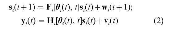
where s_i(t) is the q-variate factor or state process of system i at measurement occasion t, F_i is the matrix of autoregression coefficients relating s_i(t + 1) to s_i(t), and H_i is the matrix of loadings at t. Specific version of this linear model underlie both longitudinal factor analysis (Joreskog 1979) and dynamic factor analysis of time series (Molenaar 1994). Statistical analysis of Eqn. (2) proceeds as for Eqn. (1), although the linear state– space system Eqn. (2) allows for an analysis using standard structural equation modeling techniques.

2. System Stability

Modern concepts of system stability characterize the ways in which the internal relationships between the components of a system react to endogenous parametric changes in θ_i(t). The analysis of this so-called structural stability constituted a milestone in the nonlinear dynamics paradigm which was initiated by three scientific theories: catastrophe theory, non- equilibrium thermodynamics, and synergism. Despite differences between the three theories, they share a basic focus on the explanation of structural stability and self-organization in nonlinear systems.

Consider a system S that can vary along n dimensions. Take, for instance, a network of n artificial neurons, where the activity of each neuron constitutes a dimension along which the network can vary in time.

Then the state of S at each time point is described by an n-dimensional vector s_S(t) composed of the configuration of activity values along the n dimensions. Moreover the set of all possible values of the state across all time points constitutes the state space. Some states, i.e., some locations in state space, are special in that the system stays there if there are no perturbations. These special states are the equilibrium states of the system. From a geometrical point of view each equilibrium state acts as an attractor for those fluctuating states that are located in its domain of attraction in state space. Hence the set of equilibrium states yields a qualitative characterization of S in that it induces an organization of the state space in the form of a geometrical structure of domains of attraction.

The time-dependent changes of S are described by an n-dimensional evolution equation like Eqn. (1) in which the parameter θ_S(t) is associated with the strength of the connections between each pair of neurons. It is a defining characteristic of θ_S(t) that it changes in time at a much slower rate than the rate of change of the state s_S(t). Moreover the standard assumption is that the slow time-dependent changes of θ_S(t) are smooth, i.e., without sudden jumps.

The equilibrium states of S are defined as the states for which the rate of change as described by Eqn. (1) is zero. Consequently, the equilibrium states constitute the roots of Eqn. (1). As Eqn. (1) depends upon θ_S(t), it follows that the equilibrium states of S also depend upon θ_S(t). Hence it is evident that the set of equilibrium states will change if θ_S(t) changes. The important question in assessing structural stability is, in what way these equilibria will change. More specifically, given that θ_S(t) changes in a slow and smooth way, does this cause the set of equilibrium states to change in a similar slow and smooth way? It turns out that this depends upon the functional form of Eqn. (1): if f_S[s_S(t), θ_S(t), t] is a linear function than smooth variation of θ_S(t) always causes smooth changes in the set of equilibria of S (i.e., smooth changes in the topological pattern of domains of attraction in its state space). But if f_S[s_S(t), θ_S(t), t] is a nonlinear function then smooth variation of θ_S(t) can give rise to abrupt qualitative changes in the set of equilibria of S which can be likened to sudden earthquakes that completely reorganize the existing topological pattern of domains of attraction in its state space. That is, existing equilibria may disappear or change in character, and new types of equilibria may suddenly emerge. Such abrupt qualitative changes in the equilibria as a result of smooth parameter changes are called bifurcations (in mathematics), phase transitions (in physics), or stage transitions (in biology and psychology).

It might seem that a bifurcation originates from the smooth variation of the system parameter θ_S(t). But that can only be so in a restricted sense because smooth parameter variation belongs to a different category than the sudden qualitative changes characterizing a bifurcation. Smooth parameter variation is necessary for a bifurcation to occur, but it is not sufficient. Moreover, the action of the parameter variation in θ_S(t) is nonspecific in that the process according to which it varies does not determine the kind of qualitative changes of the equilibria of S during a bifurcation. Hence parameter variation is not a formative cause of the ensuing bifurcation. In contrast, it is the dynamical behavior of S, described by f_S, that constitutes the true formative cause of the abrupt qualitative changes in its equilibrium states. The dynamical behavior of S defines a trajectory in the same state space to which also the equilibrium states of S belong. Hence the reorganization of the topographical pattern of domains of attraction in state-space associated with a bifurcation constitutes self-organization, i.e., it is due to the formative action of the dynamics of S itself.

Analysis of structural stability of systems like S shows that nonlinear dynamical systems have the capacity to self-organize: the existing organization of their dynamical behavior transforms into qualitatively new organizations with emergent properties. This is a general mathematical result that in principle applies to any nonlinear dynamical system. In the context of developmental systems it is evident that the mathematical theory of structural stability and self-organization matches the characteristics of epigenetic processes. Epigenesis is the context-dependent un- folding of genetic control of development. In theoretical accounts this context-dependent unfolding of genetic control gives rise to stagewise developmental processes (cf. Molenaar and Raijmakers 2000, for elaboration of this point).

In mathematical analyses of bifurcations it is taken for granted that the details in Eqn. (1) describing a system are known. While this requirement will usually be met in applications in physics, it should be acknowledged that at present such detailed knowledge is lacking for most biological, behavioral and social systems. However, for a class of bifurcations called elementary catastrophes (Gilmore 1981) the analysis can proceed without specification of Eqn. (1). This makes catastrophe theory of unique importance to the analysis of structural stability, self-organization and epigenesis in biology and psychology. Van der Maas and Molenaar ( 1992) discuss in detail the application of catastrophe theory to the detection and classification of cognitive stage transitions. They present a set of inductive criteria, the so-called catastrophe flags, which provide the necessary methodological tools to establish empirically the presence of genuine stage transitions and to distinguish these from alternative developmental scenarios like sudden changes (spurts) in the level of equilibrium states due, for instance, to changes in environmental influences or the switching on or off of genetic influences. Some applications and elaborations of catastrophe analysis can be found in van der Maas and Molenaar ( 1992) and Raijmakers et al. (1996).

3. Homeostasis

Homeostasis refers to a general principle that safeguards the stability of natural and artificial systems, where stability is understood in its more classical sense of robustness against external perturbations. Homeostasis is a fundamental concept in neuropsychology, psychophysiology and neuroscience (Cannon’s thesis). In the behavioral sciences, however, the concept of homeostasis is acknowledged, but it rarely fulfils a prominent role in actual analyses. A noteworthy exception is the monograph by McFarland (1971). Yet the mathematical-statistical theory of homeostasis, in particular optimal control theory of systems with feedback (e.g., Goodwin and Sin 1984), shows that homeostasis has important effects on system behavior and hence should be taken into account in statistical system modeling and analysis. Molenaar (1987) gives an application of optimal control theory to the optimization of a psychotherapeutic process.

A concise illustration is given of some of the effects of homeostasis in applied systems modeling. Homeostasis will be defined as negative feedback control (McFarland 1971). It is shown by means of a simple computer simulation that the presence of homeostasis has profound effects on measured intercorrelations between the behavior of coupled systems. Although the systems are strongly coupled, the manifest intercorrelations between their behavior approaches zero as a direct function of the strength of homeostasis. This has noteworthy implications for applied behavioral systems analysis. Consider, for instance, the long-standing research tradition investigating the biological basis (a physiological system) of personality (a behavioral system). Both systems are assumed to be coupled, but both have also to be considered as being homeostatic. The homeostatic nature of the coupled physiological and behavioral systems investigated in this research tradition therefore can be expected to yield biased measures of their coupling (i.e., intercorrelations close to zero), whereas the actual strength of this coupling may be considerable.

The illustrative simulation study is based on a simple instance of the linear state–space model in Eqn. (2). Only a single set of two coupled systems is considered, hence the subscript i can be dropped in the defining equations. To simplify matters further, it is assumed that the state s(t) is observed directly, hence the matrix H is taken to be the identity matrix and the measurement noise v(t) is absent. Denoting the unidimensional state process of system 1 (e.g., the behavioral system) by s₁(t) and the unidimensional state process of system 2 (e.g., the physiological system) by s₂(t), this yields:

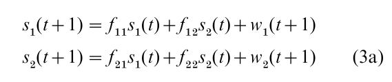
In Eqn. (3a) f₁s₂(t) denotes the influence of the physiological system on the behavioral state process s₁ (t + 1), where f₁₂ is the strength of this coupling; f₂₁s₁(t) denotes the reverse influence of the behavioral system on the physiological state process s₂(t + 1).

The system Eqn. (3a) does not include homeostasis. In contrast, the following analogue of Eqn. (3a) includes homeostasis:

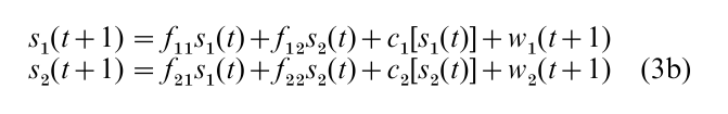
In Eqn. (3b) c₁[s₁(t)] and c₂[s₂(t)] denote optimal feedback functions which depend on a number of additional parameters that are not displayed explicitly. Molenaar (1987, and references therein) presents a complete description of the computation of these optimal feedback functions.

To assess the effects of homeostasis on the manifest correlation between s₁(t) and s₂(t), time series are generated according to Eqns. (3a) and (3b). This requires that numerical values are assigned to the system parameters in both Eqns. (3a) and (3b). For instance: f₁₁ = 0.6, f₁₂ = 0.4, f₂₁ = 0.4, and f₂₂ = 0.7. In addition, c₁[s₁(t)] is taken to be zero (only the physiological system 2 in (3b) includes homeostasis). It is then found that the manifest instantaneous intercorrelation between s₁ (t) and s₂ (t), as determined for a realization of T = 100 time points, is 0.85 for Eqn. (3a) and 0.15 for Eqn. (3b). This shows clearly that the intercorrelation for Eqn. (3b), that is when homeostasis is present in the physiological system 2, is substantially biased towards zero and does not reflect the strength of the coupling between the two systems without homeostasis present.

The same result (substantial underestimation of the actual coupling strength by the manifest intercorrelation between coupled systems in case homeostasis is present) is found under all other possible scenarios (negative coupling between systems without homeostasis, homeostasis present in both systems, etc.). This general result also can be proven by means of mathematical-statistical methods. It is concluded that homeostasis has substantial biasing effects on manifest measures of system coupling, even in simple linear systems such as considered above.

4. Wholeness And Individuality

The slogan that the whole is more than its parts implies that distinct systems may each be composed of the same set of components, yet still be different from each other in their global characteristics of systemhood. Another way to state this point of view is that the unity characterizing each system gives rise to emergent characteristics, and thus to individuality.

To investigate the individuality of a given system i, it is required to observe its time-dependent behavior y_S(t), t = 1, 2, …, T, at T consecutive time points (where, to simplify the discussion, consecutive time points are taken to be equidistant). Hence S is fixed and the time interval from t = 1 to t = T is conceived of as a sample from the time axis. With regard to Eqn. (1) and Eqn. (2), this implies that i = S is taken to be fixed, whereas statistics and parameter estimates are determined by taking appropriate averages over time points, and consecutively are generalized to the whole time axis (prediction and retrodiction). Henceforth this (N = 1 time series) design will be called an analysis of intra-individual variation (IAV).

If a set (population) of systems can be taken to be homogeneous in all relevant aspects, then their time-dependent behavior can be analyzed in the following way: take a sample of N systems from the set and observe the time-dependent behavior y_i(t_j), i = 1, …, N of this sample at a fixed set of time points t_j, j = 1, …, J. Hence, with regard to Eqns. (1) and (2) the J time points are fixed, whereas statistics and parameter estimates are determined by taking appropriate averages over systems, and consecutively are generalized to the whole set or population of systems. Henceforth this (longitudinal) design will be called an analysis of inter-individual variation (IIV).

The particular aspect of wholeness and individuality of systems which will concern us in this section can now be stated more specifically as: under which circumstances and conditions will a longitudinal analysis of IIV yield results that are qualitatively the same as a time series analysis of IAV? This question can be raised with respect to all known techniques of statistical analysis, like analysis of variance, regression analysis, factor analysis, etc. In what follows, only factor analysis is considered in the context of the linear model in Eqn. (2), leading to the particular question: given that y consists of a fixed set of manifest variables (e.g., psychological test scores), under which circumstances will a longitudinal factor analysis of y_i(t_j) yield results that are qualitatively the same (same number of latent factors, same pattern of factor loadings, etc.) as a dynamic factor analysis of y_S(t)? For more extensive elaboration of this issue, the reader is referred to Molenaar et al. (2001).

The mathematical-statistical ergodicity theory is of direct relevance to this question. Ergodicity is a basic concept in statistical mechanics and equilibrium thermodynamics (e.g., Cornfield et al. 1982). Consider a closed domain containing a pure gas, where each gas molecule traverses a path or trajectory according to standard dynamical laws. The totality of these time- dependent trajectories of all gas molecules within the domain constitutes an ensemble (comparable with the concept of population in statistics). The dynamics of this ensemble is called ergodic if statistics like the mean velocity determined by following a single molecule in time is (asymptotically) the same as the mean velocity determined by averaging across all molecules at a fixed point in time. Notice that this closely parallels the basic issue under consideration: a process is ergodic if analysis of its IAV yields the same results as an analysis of its IIV. In contrast, if a process is nonergodic then this equivalence no longer holds. A heuristic criterion for ergodicity which applies in many cases is that the mean, variance and covariance associated with an ergodic process are invariant in time. With respect to Eqn. (2) this ergodicity criterion implies that F_i[θ_i(t), t] = F_i[θ_i] and H_i[θ_i(t), t] = H_i[θ_i], i.e., these matrices (as well as the parameter vector θi) have to be invariant in time.

The ergodicity question is an important issue in theoretical discussions in developmental psychology (cf. Molenaar et al. 2001). If developmental psychology is conceived of as the study of ontogenetic trajectories across the lifespan, then the life history of each individual subject constitutes a path in some high-dimensional state–space, while a population of subjects defines an ensemble of such age-dependent paths. The theoretical debate concerns the question whether the pattern of IIV within such an ensemble of life histories at some point in time contains sufficient information to arrive at valid causal explanations of the pattern of IAV characterizing the time course of each individual life history (cf. Wohlwill 1973).

The ergodicity question also is relevant to the foundations of psychometrics. Standard (longitudinal) factor analysis is the classical method to construct psychological tests (Lord and Novick 1968). Now suppose that it has been concluded in a longitudinal factor analysis that a particular psychological test obeys a 1-factor model at each measurement occasion, that the factor loadings stay invariant across measurement occasions, and that the intercorrelations of factor scores between measurement occasions are high. Hence the structure of interindividual variation of the scores on this test is simple: it stays qualitatively the same across measurement occasions and is characterized by high stability. If this particular test is used in a clinical or counseling setting to predict the scores of a single subject belonging to the population from which the longitudinal sample was drawn, can we be sure that this simple structure also characterizes this subject’s IAV? More specifically, can we expect to find in a dynamic factor analysis of this single subject’s scores also a 1-dimensional dynamic factor which stays qualitatively invariant in time and has high stability? If the test is measuring a nonergodic process then the answer will be negative.

The consequences of nonergodicity can be observed clearly in classical test theory. Lord and Novick (1968) define the basic concept of true score as the mean of the intraindividual distribution of scores of a fixed subject. Then they remark (Lord and Novick 1968, p. 32): ‘The true and error scores defined above are not those primarily considered in test theory. They are, however, those that would be of interest to a theory that deals with individuals rather than with groups (counseling rather than selection).’ Next, instead of defining true and error scores for a single fixed person tested an arbitrarily large number of times, true and error scores are defined for an arbitrarily large number of persons tested at one or more fixed times. Hence, instead of focusing on IAV as stipulated by the initial definition of true score, classical test theory is based on IIV. The quote from Lord and Novick given above clearly indicates the restricted nature of results thus obtained in classical test theory.

The standard longitudinal factor model is a special instance of Eqn. (2) in which F_i[θ_i(t), t] = F[θ(t), t] and H_i[θ_i(t), t] = H[θ(t), t]. That is, these matrices as well as the parameter vector are taken to be invariant across systems (subjects), but may vary in time. Comparison with the heuristic criterion for ergodicity given earlier (i.e., F_i[θ_i(t), t] = F_i[θ_i] and H_i[θ_i(t), t] = H_i[θ_i]), it is immediately evident that the possible time- dependency of F[θ(t), t], H[θ(t), t] and θ(t) in the longitudinal factor model implies the possibility of nonergodicity. Hence in general the structure of IIV as determined in standard longitudinal factor analysis (e.g., test–retest designs) will differ from the structure of IAV as determined in dynamic factor analysis. In particular, psychological tests which have been constructed and normed by means of test–retest factor analysis will in general yield invalid assessments and predictions in individual counseling. This is a straightforward consequence of classical theorems in ergodicity theory.

It also is evident that the assumptions underlying standard (longitudinal) factor analysis regarding the invariance of the F and H matrices across systems (subjects) would seem to be a odds with the individuality and wholeness of systems as considered in this section. There is strong theoretical and empirical evidence that in many circumstances systems (subjects) do not obey these strong homogeneity assumptions and instead are heterogeneous, i.e., Fi, Hi and θi vary across systems i. It can be proven that (longitudinal) factor analysis is in general insensitive to this kind of heterogeneity, despite its incompatibility with the homogeneity assumptions underlying this analysis. This insensitivity has been corroborated in several simulation studies using the following design. An ensemble of individual time-dependent trajectories (life histories) y_i(t), t = 1, 2, …, T, i = 1, 2, …, N, is generated according to dynamic factor models with heterogeneous system matrices and parameter vectors varying across systems (subjects). Then (longitudinal) factor analysis is carried out on a sample from this ensemble at one or more fixed time points. The consistent finding then is, that 1-factor (longitudinal) models yield satisfactory fits to these data, while the structure and parameter estimates in the fitted models do not match any of the structures and parameters in the dynamic factor model used to generate the data (cf. Molenaar et al. 2001, for details and references).

5. Conclusion

Aspects of systemhood can have profound implications for the modeling and analysis of social, behavioral and biological systems. This has been illustrated by a consideration of three such aspects: structural stability (emergent changes in the geometry of (strange) attractors in state–space), homeostasis (negative feedback inducing underestimation of system coupling), and wholeness (nonergodicity inducing a lack of relationship between analyses of IAV and IIV). Each of these aspects can be underpinned by powerful mathematical-statistical theories and has been studied in extensive simulation studies, showing their manifold effects on system modeling. It is concluded that to accommodate the effects of systemhood in valid ways, advanced time series analysis techniques will prove to be indispensable.

Bibliography:

1. Cornfield I P, Fomin S V, Sinai Y G 1982 Ergodic Theory. Springer, New York
2. Elliott R J, Aggoun L, Moore J B 1995 Hidden Marko Models: Estimation and Control. Springer, New York
3. Gilmore R 1981 Catastrophe Theory for Scientists and Engineers. Wiley, New York
4. Goodwin G C, Sin K S 1984 Adaptive Filtering, Prediction and Control. Prentice-Hall, Englewood Cliffs, NJ
5. Joreskog K G 1979 Statistical estimation of structural models in longitudinal developmental investigations. In: Nesselroade J R, Baltes P B (eds.) Longitudinal Research in the Study of Behavior and Development. Academic Press, New York, pp. 303–51
6. Klir G J 1991 Facets of System Science. Plenum, New York
7. Lord F M, Novick M R 1968 Statistical Theories of Mental Test Scores. Addison-Wesley, Reading, MA
8. McFarland D J 1971 Feedback Mechanisms in Animal Behaviour. Academic Press, London
9. Molenaar P C M 1987 Dynamic assessment and adaptive optimisation of the therapeutic process. Behavioral Assessment 9: 389–416
10. Molenaar P C M 1994 Dynamic latent variable models in developmental psychology. In: von Eye A, Clogg C C (eds.) Latent Variable Analysis: Applications for Developmental Research. Sage, Newbury Park, CA, pp. 155–80
11. Molenaar P C M, Raijmakers M E J 2000 A causal interpretation of Piaget’s theory of cognitive development: Reflections on the relationship between epigenesis and nonlinear dynamics. New Ideas in Psychology 18: 41–55
12. Molenaar P C M, Huizenga H M, Nesselroade J R 2001 The relationship between the structure of inter-individual and intra-individual variability: A theoretical and empirical vindication of developmental systems theory. In: Staudinger U M, Lindenberger U (eds.) Understanding Human Development
13. Raijmakers M E J, van Kooten S, Molenaar P C M 1996 On the validity of simulating stagewise development by means of PDP networks: Application of catastrophe analysis and an experimental test of rule-like network performance. Cognitive Science 20: 101–36
14. Van der Maas H L J, Molenaar P C M 1992 Stagewise cognitive development: An application of catastrophe theory. Psychological Review 99: 395–417
15. Wohlwill J F 1973 The Study of Development. Academic Press, New York