Order Statistics Research Paper

1. Introduction

Let the variates X₁, …, X_n be arranged in ascending order and written X_1:n ≤ X_r:n ≤…≤ =X_n:n. Then X_r:n is the rth order statistic (r = 1, …, n), a term also applied to the corresponding observed value, x_r:n. The median is X_(n+1)/2:n for n odd and 1/2(X_n/2:n + X_n/2+1:n) for n even. Helped by their simplicity, the median and the range, X_n:n – X_1:n, have long been valuable as measures of location and scale, respectively.

Consider the following illustrative data, with i = 1, …, 8

x_i:      16        40        23        12        240      33        17        27

x_i:8:   12        16        17        23        27        33        40        240

These figures may represent the annual incomes (in multiples of $1,000) at age 30 of eight high-school dropouts. Because of the outlier x₅ = 240, the median, 1/2(23 + 27) = 25, clearly gives a better picture of the group than the mean, 51. The median would in fact be unchanged as long as x₅ ≥ 27, which shows just how robust the median is.

Next, suppose that the xi are test scores out of a total of 40. If we are unable to correct the impossible score of 240, we eliminate or censor it. The median is then x_4:7 = 23, no longer very different from the mean, x = 24. The range is not robust, dropping from 228 to 28, and is therefore useful in detecting outliers, which are seldom as obvious as in the above data (see Sect. 6.3). For ‘well-behaved’ data, the range provides a simple measure of variability or scale.

In time series, X₁, X₂, …, these descriptive statistics are particularly helpful when based on small moving subsamples X_j, X_j+1, …, X_j+n−1 ( j = 1,2, …). The resulting moving (or running) medians provide a current measure of location that, unlike the moving mean, is not too sensitive to outliers. The sequence of moving medians represents a smoothing of the data, with important applications in signal and image processing. Moving ranges are useful in quality control charts, where their sensitivity to outliers is a desirable feature. If more robust current estimators of dispersion are required, one can turn to the difference of the second largest and the second smallest in each moving sample, etc.

Again, the above xi may represent response times to a stimulus. The extremes, 12 and 240, are then of particular interest (see Sect. 5.2). Of course, we would want more extensive data for which we may also wish to study the upper and lower records, here (16, 40, 240) and (16, 12).

2. Basic Distribution Theory

If X₁, …, X_n is a random sample from a population with cumulative distribution function (cdf ) F(x), then the cdf of X_r:n is given by

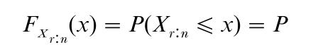
 (at least r of X₁, …, X_n are less than or equal to x)

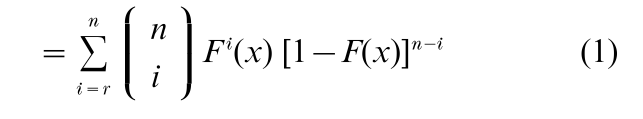
since the term in the summand is the binomial probability that exactly i of X₁, …, X_n are less than or equal to x.

In handling order statistics, usually it is assumed that the underlying variate X is continuous. Note that this assumption is not needed in the derivation of Equation (1). Also, if X can take only integral values, then P(X_r:n = x) = F_Xr:n(x) – F_Xr:n(x – 1). However, if X is discrete, the probability of ties among the observations is positive, which tends to complicate the distribution theory (see, e.g., David 1981, p. 13, Arnold et al. 1992, p. 41).

If the probability density function (pdf)f (x) exists, as we will assume from here on, then differentiation of Eqn. (1) yields

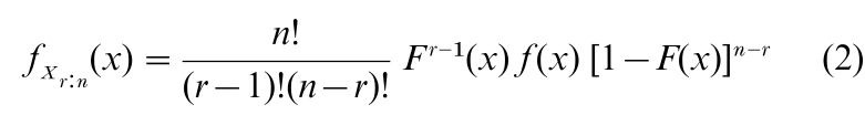
Also, the joint pdf of X_r:n and X_s:n (1 ≤ r < s ≤ n) is, for x ≤ y (e.g., David 1981, p. 10, Arnold et al. 1992, p. 16)

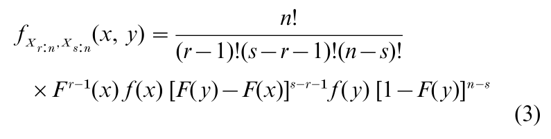
Equations (2) and (3) are fundamental and permit the calculation, usually by numerical integration, of the means, variances, and covariances. Also, Eqn. (3) makes possible the derivation, by standard methods, of the pdf of functions of two order statistics, such as the range W_n = X_n:n – X_1:n. To facilitate the use of order statistics, extensive tables have been developed, especially when F(x) = Φ(x), the standard normal cdf (see Pearson and Hartley 1970 1972, Harter and Balakrishnan 1996, 1997).

3. Distribution-Free Inter Al Estimation

Three important types of distribution-free intervals involving order statistics may be distinguished. For simplicity we assume that F(x) is strictly increasing for 0 < F(x) < 1.

3.1 Confidence Intervals For Quantiles

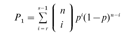
The (population) quantile of order p, ξ_p, is defined by F(ξ_p) = p, 0 < p < 1. In particular, ξ_1/2 is the median. Since, for r < s P(X_r:n < ξ_p < X_s:n) = P(X_r:n < ξ_p) – P(X_s:n < ξ_p), it follows from Eqn. (1) that the interval (X_r:n, X_s:n) covers ξ_p with probability

3.2 Tolerance Intervals

The focus here is on the probability, P₂, with which (X_r:n, X_s:n) covers a proportion γ of the underlying population. Thus P₂ = P{F(X_s:n) – F(X_r:n) ≥ γ} Since F(X ) is a uniform (0,1) variate, U, P₂ = P (U_s:n – U_r:n ≥ γ) = 1 – I_γ(s – r, n – s + r + 1), with the help of Equation (3), where I_γ (a,b) is the incomplete beta function.

3.3 Prediction Intervals

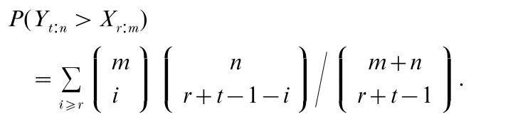
Let X₁, …, X_m, Y₁, …, Y_n be independent variates with cdf F(x). The Xs may represent current observations and the Ys future observations. What is the probability, P , that Y_t:n (t = 1, …, n) falls between X_r:m and X_s:m (1 ≤ r < s ≤ m)? It can be shown that P₃ = P(Y_t:n > X_r:m) – P(Y_t:n > X_s:m), where

A good account from the user’s point of view of all these intervals is given in Chap. 5 of Hahn and Meeker (1991).

4. Estimation Of Parameters

An important simple example is the use of range in quality control to estimate the standard deviation (sd) σ in a normal sample. If w_n;α denotes the upper α significance point of the range in a standard normal population, then from P(w_n;1−a/2 < W_n/σ < w_n;a/2) = 1 – α it follows that a (1 – α) confidence interval (CI) for σ is

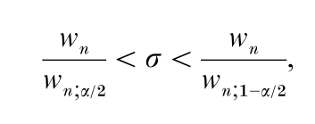
where w_n is the observed value of the range.

An unbiased point estimator of σ is σ_W = W_n /d_n, where d_n = E(W_n/σ) is widely tabulated. Let σ_S denote the unbiased root-mean-square estimator of σ. In small samples the efficiency of σ_W, i.e., var σ_S/ var σ_W, is quite high (0.955 for n 5).

More systematically, linear functions of the order statistics (L-statistics) can be used to estimate both location and scale parameters, µ and σ (not necessarily mean and sd), for distributions with pdf of the form

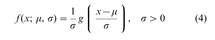
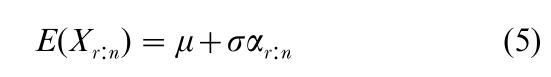
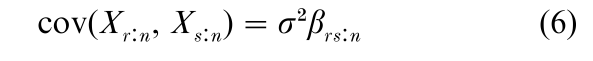
With Y = (X – µ)/σ, let α_r:n = E (Y_r:n) and β_rs:n = cov (Y_r:n, Y_s:n) (r, s = 1, …, n). It follows that X_r:n = µ + σY_r:n, so that

A major advance was made by Lloyd (1952), who recognized that the generalized Gauss–Markov theorem can be applied to the estimation of µ and σ, in view of Eqns. (5) and (6). This yields the best linear unbiased estimators (BLUEs).

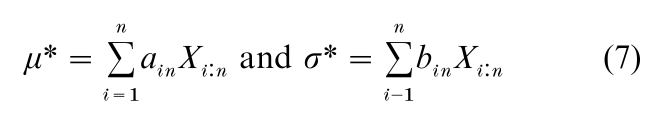
where the a_in and bin are functions of the α_i:n and β_ij:n and can be evaluated once and for all. For tables in the normal case, see Sarhan and Greenberg (1962).

The statistics in Eqn. in (7) provide estimators that are unbiased and of minimum variance within the class of linear unbiased estimators. They are particularly convenient for data in which some of the smallest and/or largest observations have been censored, since maximum likelihood (ML) estimation tends to be difficult in this situation. Also, for complete and censored samples, ML estimation may produce biased estimators. However, µ* and σ* may not have the smallest mean squared error, even among L- statistics. Simplified approximate estimation procedures are also possible (see, e.g., David 1981, p. 128 or Arnold et al. 1992, p. 171).

5. Asymptotic Theory

Except for the distribution-free results of Sect. 2, the practical use of order statistics in finite samples depends heavily on the availability of tables or computer programs appropriate for the underlying population. In large samples, asymptotic theory can provide approximate results that are both simpler and more widely applicable.

It is useful to distinguish three situations as n → ∞: (a) Central order statistics X_(np):n, where (np) denotes here the largest integer ≤ np + 1, with 0 < p < 1; (b) Extreme order statistics X_r:n, where r = 1, …, m or r = n – m + 1, …n, and m is a fixed positive integer; (c) Intermediate order statistics X_r:n or X_n−r+1:n, where r → ∞ but r/n → 0.

5.1 Central Order Statistics

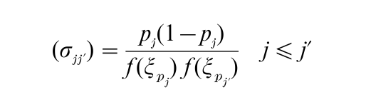
Corresponding to the population quantile ξ_p of Sect. 2.1, it is natural to call X_(np):n a sample quantile. The following important result then holds (e.g., David 1981, p. 254). Let X₁, …, X_n be a random sample from a population with pdf f (x) and put n_j = (np_j), j = 1, …, k, where k is fixed and 0 < p₁ < p₂ <…< p_k < 1. If 0 < p(ξ_pj) < ∞, j = 1, …, k, then the asymptotic joint distribution of √n(X_{n :n} – ξ_p1), …, √n(X_nk:n -ξ_pk) is k-dimensional normal, with zero mean vector and covariance matrix (σ_jj), where

As a very special case, it follows that for the median M_n = X_(n+1)/2:n (n odd), as n → ∞, √n(M_n – µ) → N (0, πσ²/2) showing incidentally that, as an estimator of µ, M_n has asymptotic efficiency (relative to X ) of 2/π = 0.637. The same result holds for n even.

5.2 Extreme Order Statistics

The situation is more complicated when p₁ = 0 or p_k = 1, corresponding to the extremes X_1:n, X_n:n and more generally to the mth extremes X_m:n, X_n+1−m:n, where m is a fixed positive integer. For X_n:n, suitably normalized, there are three limiting distributions, the simplest of which is the Type III extreme-value distribution with cdf Λ₃(x) = exp (-e^−x) – ∞ < x < ∞. This distribution has been found very useful in describing the behavior of floods and other extreme meteorological phenomena. A convenient sufficient condition for Λ₃(x) to be the appropriate limiting distribution is that the underlying distribution satisfy

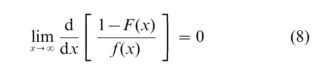
Then

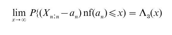
where an is given by F(a_n) = 1 – 1/n. Distributions for which Eqn. (8) holds include the normal, gamma, and logistic families. For a full treatment of the extreme-value case, see Galambos (1987).

5.3 Intermediate Order Statistics

An example of an intermediate order statistic is X_√n:n. A suitably normalized form of X_r:n may have either a normal or nonnormal asymptotic distribution (e.g., Arnold et al. 1992, p. 226).

5.4 Asymptotic Independence Results

A useful result is that, after appropriate normalization, upper extremes are asymptotically independent of lower extremes. Moreover, all extremes are asymptotically independent of the sample mean (e.g., David 1981, pp. 267–70).

5.5 L-Statistics

It is clear from the above that a linear function of sample quantiles, ∑^k_j=1c_jX_nj:n, tends to normality as n → ∞ (k fixed). On the other hand, the asymptotic distribution of linear functions of the extremes, such as the range, will be more complicated. An L-statistic, ∑ⁿ_i=1c_inX_i:n, involving extreme, intermediate, and central order statistics, may be asymptotically normal or nonnormal, depending on the underlying distribution and on how much weight is placed on the extreme order statistics.

6. Applications

6.1 Probability Plotting

This very useful graphical method typically is applied to data assumed to follow a distribution depending, as in Eqn. (3), only on location and scale parameters µ and σ. The ordered observations x_i:n(i = 1, …, n) are plotted against ν_i = G⁻¹ ( p_i), where G is the cdf of Y = (X – µ) σ and the p_i are probability levels, such as p_i =(i – 1/2)/n. The plotting is immediate if probability paper corresponding to G is available, as it is for, for example, the normal, lognormal, and Weibull distributions. If a straight-line fit through the points (ν_i, x_i:n) seems unreasonable, doubt is cast on the appropriateness of G. Often this simple procedure is adequate, but it may be followed up by a more for- mal test of goodness-of-fit.

If a straight line fits satisfactorily, a second use may be made of the graph: σ may be estimated by the slope of the line and µ by its intercept on the vertical axis. A detailed account of probability plotting and the related hazard plotting is given in Nelson (1982).

6.2 Selection Differentials And Concomitants Of Order Statistics

If the top k ( < n) individuals are chosen in a sample from a population with mean µ and sd σ, then D_k,n = (X_n−k+1:n +…+ X_n:n – k_µ)/kσ measures the superiority, in sd units, of the selected group. The mean and variance of this selection differential is given immediately by Eqns. (5) and (6) as E (D_k,n) = ∑ _αi:n /k, var (D_k,n) =∑∑β_ij:n/k², where all summations run from n – k + 1 to n.

Often one is interested in how this group performs on some related measurement Y. Thus, X may refer to a screening test and Y to a later test or X to a parent animal and Y to an offspring. The Y-variate paired with X_r:n may be denoted by Y_[r:n] and called the concomitant of the rth order statistic. Corresponding to D_k,n, the superiority of the selected group on the Y-measurement is, with obvious notation, D_[k,n] = (∑Y_[i:n] – kµ_Y)/kσ_Y. If Y is linearly related to X, such that Y_i = µ_Y + ρσ_Y(X_i – µ_X)/σ_X + Z_i where ρ is the correlation coefficient between X and Y, and Z_i is independent of X_i, with mean 0 and variance σ_Y²(1 – ρ²), then Y_[r:n] = µ_Y + ρσ_Y(X_r:n – µ_X)/σ_X + Z_[r] where Z_[r] is the Z-variate associated with X_r:n (e.g., David 1981, p.110 ). It follows that EY_r:n = µ_Y + ρσ_Yα_r:n, var Y_[r:n] = σ²_Y(ρ²β_rr:n + 1 – ρ²), cov (Y_[r:n], Y_[s:n]) = ρ²σ²_Yβ_rs:n r =s so that the mean and variance of D_[k,n], the induced selection differential, are ED_[k,n] = ρED_k:n, var D_[k,n] = ρ²var D_k:n + (1 – ρ² )/k. The asymptotic distribution of D^[k:n] as well as many other properties and applications of concomitants of order statistics are treated in David and Nagaraja (1998).

6.3 Outliers And Selection Of The Best

Order statistics, especially X_n:n and X_1:n, enter naturally into many outlier tests. Thus, if X₁, …, X_n are supposedly a random sample from a normal dis tribution with unknown mean and known variance σ², then large values of B_n = (X_n:n – X)/σ make this null hypothesis, H₀ , suspect. The corresponding two-sided statistic is B_n´ = ^max_i=1,…,n|X_i-X|σ . If σ is unknown, studentized versions of B_n or B_n´ can be used. The subject, with its many ramifications, is treated extensively in Barnett and Lewis (1994), where tables needed to carry out such tests are given. If the observed value of the chosen statistic is large enough, H₀ is rejected and X_n:n (or X_1:n) becomes a candidate for further examination or rejection.

The foregoing approach is related closely to the following multiple decision procedure, illustrated on the balanced one-way classification with n ‘treatment’ means X_i, i = 1, …, n, each based on m replications. To test the null hypothesis H₀ of equal population means µ₁, …, µ_n against the ‘slippage’ alternative µ₁ =…=µ_i−1 = µ_i+1 =…µ_n and µ_i = µ₁ + ∆, where i and ∆ < 0 are unknown, n + 1 decisions may be taken, that is, D₀:H₀ holds or D_i: the ith treatment mean has slipped to the right. Under the usual normal-theory assumptions, an optimal procedure at significance level α is to choose D_M if / (e.g., David 1981, p. 226) C_n,ν = m (X_M – X )/(TSS)^1/2 > c_n,υ;α, where M is the subscript corresponding to the largest X_i, TSS is the analysis of variance total sum of squares, and c_n,v;α, with ν = n(m – 1), is given in Table 26a of Pearson and Hartley (1970 1972). If C_n,υ < c_n,υ;α the decision D is taken. Slippage in either direction can be handled similarly with Table 26b.

In the above, the focus is on the detection of a single outlier or a single superior (or inferior) treatment. The handling of multiple outliers is an important part of Barnett and Lewis (1994).

6.4 Simultaneous Inference

Order statistics play an important supporting role in simultaneous inference procedures. A well-known example is Tukey’s use of the studentized range in setting simultaneous confidence intervals for the treatment means in fixed-effects balanced designs.

6.5 Robust Estimation

Here one gives up the classical idea of using an estimator that is optimal under tightly specified conditions in favor of an estimator that retains reasonably good properties under a variety of departures from the hypothesized situation. Since the largest and smallest observations tend to be more influenced by such departures, which include the presence of outliers, many robust procedures are based on the more central order statistics. A simple example is provided by the trimmed means

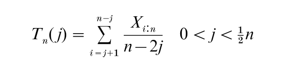
which include the sample median as a special case. For a very readable treatment of robust methods see Hoaglin et al. (1983).

6.6 Data Compression And Optimal Spacing

Given a large random sample of size n from a population with pdf, Eqn. (4), it is possible to estimate µ or σ or both from a fixed small number k of well chosen order statistics. The loss in efficiency of estimation may be more than compensated by the storage space gained, especially as a test of the assumed underlying distribution can still be made by probability plotting. For example, in the case of a normal population, the optimal estimator of µ is, for k = 4,

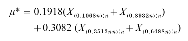
where (0.1068n) is the largest integer ≤ 0.1068n +1, etc. The estimator µ* has asymptotic efficiency (AE) 0.920 and, since it does not involve the more extreme order statistics, is more robust than X. Also, µ* is much more efficient than the median (AE = 0.637) (see, e.g., David 1981, Sect. 7.6).

7. Concluding Remarks

The two large multiauthored volumes (Balakrishnan and Rao 1998a, 1998b) cover many more topics in both theory and applications of order statistics than can even be mentioned here. Additional applications include ranked set sampling and especially the use of median, order-statistic, and other filters in signal and image processing.

Bibliography:

1. Arnold B C, Balakrishnan N, Nagaraja H N 1992 A First Course in Order Statistics. Wiley, New York
2. Balakrishnan N, Rao C R (eds.) 1998a Handbook of Statistics 16, Order Statistics: Theory & Methods. Elsevier, Amsterdam
3. Balakrishnan N, Rao C R (eds.) 1998b Handbook of Statistics 17, Order Statistics: Applications. Elsevier, Amsterdam
4. Barnett V, Lewis T 1994 Outliers in Statistical Data, 3rd edn. Wiley, New York
5. David H A 1981 Order Statistics, 2nd edn. Wiley, New York
6. David H A, Nagaraja H N 1998 Concomitants of Order Statistics. In: Balakrishnan N, Rao C R 1998a, (eds.) Handbook of Statistics 16, Order Statistics: Theory & Methods. Elsevier, Amsterdam, pp. 487–513
7. Galambos J 1987 The Asymptotic Theory of Extreme Order Statistics, 2nd edn. Krieger, Malabar, FL
8. Hahn G J, Meeker W Q 1991 Statistical Intervals: A Guide for Practitioners. Wiley, New York
9. Harter H L, Balakrishnan N 1996 CRC Handbook of Tables for the Use of Order Statistics in Estimation. CRC Press, Boca Raton, FL
10. Harter H L, Balakrishnan N 1997 Tables for the Use of Range and Studentized Range in Tests of Hypotheses. CRC Press, Boca Raton, FL
11. Hoaglin D C, Mosteller F, Tukey J W (eds.) 1983 Understanding Robust and Exploratory Data Analysis. Wiley, New York
12. Lloyd E H 1952 Least-squares estimation of location and scale parameters using order statistics. Biometrika 38: 88–95
13. Nelson W 1982 Applied Life Data Analysis. Wiley, New York
14. Pearson E S, Hartley H O (eds.) 1970/1972 Biometrika Tables for Statisticians, Vol. 1, 3rd edn., Vol. 2. Cambridge University Press, Cambridge, UK
15. Sarhan A E, Greenberg B G (eds.) 1962 Contributions to Order Statistics. Wiley, New York