Time Series and Economic Forecasting Research Paper

1. Time Series Models For Economic Forecasting

Broadly speaking, statistical approaches to economic forecasting fall into two categories: time-series methods and structural economic models. Time-series methods use economic theory mainly as a guide to variable selection, and rely on past patterns in the data to predict the future. In contrast, structural economic models take as a starting point formal economic theory and attempt to translate this theory into empirical relations, with parameter values either suggested by theory or estimated using historical data. In practice, time-series models tend to be small with at most a handful of variables, while structural models tend to be large, simultaneous equation systems which sometimes incorporate hundreds of variables. Time-series models typically forecast the variable(s) of interest by implicitly extrapolating past policies into the future, while structural models, because they rely on economic theory, can evaluate hypothetical policy changes. In this light, perhaps it is not surprising that time-series models typically produce forecasts as good as, or better than, far more complicated structural models. Still, it was an intellectual watershed when several studies in the 1970s (reviewed in Granger and Newbold 1986) showed that simple univariate time-series models could outforecast the large structural models of the day, a result which continues to be true (see McNees 1990). This good forecasting performance, plus the relatively low cost of developing and maintaining time-series forecasting models, makes time-series modeling an attractive way to produce baseline economic forecasts.

At a general level, time-series forecasting models can be written,

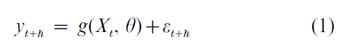
where y_t denotes the variable or variables to be forecast, t denotes the date at which the forecast is made, h is the forecast horizon, X_t denotes the variables used at date t to make the forecast, θ is a vector of parameters of the function g, and ε_t+h denotes the forecast error. The variables in X_t usually include current and lagged values of y_t. It is useful to define the forecast error in (1) such that it has conditional mean zero, that is, E(ε_t+h |X_t) = 0. Thus, given the predictor variables X_t, under mean-squared error loss the optimal forecast of y_t+h is its conditional mean, g(X_t, θ). Of course, this forecast is infeasible because in practice neither g nor θ are known. The task of the time-series forecaster therefore is to select the predictors X_t, to approximate g, and to estimate θ in such a way that the resulting forecasts are reliable and have mean-squared forecast errors as close as possible to that of the optimal infeasible forecast.

Time-series models are usefully separated into univariate and multivariate models. In univariate models, X_t consists solely of current and past values of _yt. In multivariate models, this is augmented by data on other time series observed at date t. The next subsections provide a brief survey of some leading time-series models used in economic forecasting. For simplicity attention is restricted to one-step ahead forecasts (h = 1). Here, the focus is on forecasting in a stationary environment; the issue of nonstationarity in the form of structural breaks or time varying parameters is returned to below.

1.1 Univariate Models

Univariate models can be either linear, so that g is linear in X_t, or nonlinear. All linear time-series models can be interpreted as devices for modeling the covariance structure of the data. If {y_t}, t =1, … ,T has a Gaussian distribution and if this distribution is stationary (does not depend on time), then the optimal forecast is a linear combination of past values of the data with constant weights. Different linear time-series models provide different parametric approximations to this optimal linear combination.

The leading linear models are autoregressive models, autoregressive–integrated moving-average (ARIMA) models, and unobserved components models.

An autoregressive model of order p (AR( p)) is written,

where (µ, α₁, … , α_p) are unknown parameters, L is the lag operator, and α(L) is a lag polynomial. If y_t is observed at all dates, t = 1, … , T, these parameters are readily estimated by ordinary least squares.

ARIMA models extend autoregressive models to include a moving-average term in the error, which has the effect of inducing long lags in the forecast when it is written as a function of current and past values of y_t. These are discussed in Time Series: ARIMA Methods.

In an unobserved components model, y_t is represented as the sum of two or more different stochastic components. These components are then modeled, and the combined model provides a parametric approximation to the autocovariances; see Harvey (1989) for a detailed modern treatment. The unobserved components framework can provide a useful framework for extracting cyclical components of economic time-series and for seasonal adjustment.

If {y_t} is not Gaussian, in general the optimal forecast will not be linear, which suggests the use of forecasts based on nonlinear time-series models. Parametric nonlinear time-series models posit a functional form g, and take this as known up to the finite-dimensional parameter vector θ. Two leading examples of parametric nonlinear time-series models, currently popular for economic forecasting, are threshold autoregressive models and Markov switching models. Both are similar in the sense that they posit two (or more) regimes. In the threshold autoregression, switches between the regimes occur based on past values of the observed data; in Markov switching models, the switches occur based on an unobserved or latent variable.

The threshold autoregressive family of models can be written

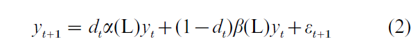
where the mean is suppressed, α(L) and β(L) are lag polynomials, and d_t is a nonlinear function of past data that switches between the ‘regimes’ α(L) and β(L). Variations of Eqn. (2) interact d_t with only some autoregressive coefficients, the intercept, and/or the error variance. Various functions are available for d_t, either a sharp indicator function (the threshold auto-regressive model) or a smooth function (smooth transition autoregression). For example, setting d_t = (1 + exp [γ₀ +γ`₁ζ_t])⁻¹, yields the logistic smooth transition autoregression (LSTAR) model, where ζ_t denotes current or past data, say, ζ_t might equal y_t−k for some k. See Granger and Terasvirta (1993) for additional details. For an application of threshold autoregressions (and other models) to forecasting US unemployment, see Montgomery et al. (1998).

The Markov switching models are conceptually similar, except that the regime switch depends on an unobserved series. In the context of Eqn. (2), d_t is modeled as unobserved and following a two-state Markov process; see Hamilton (1994).

An alternative approach is to treat g itself as unknown, which leads to nonparametric methods. These include nearest neighbor, kernel, and artificial neural network models for the conditional expectation. In practice these nonparametric approaches to economic forecasting have met with success which is mixed at best. There are several possible reasons for this, including that there are insufficiently many observations in typical economic data sets to support the use of these data-intensive methods.

1.2 Multivariate Models

In multivariate time-series models, X_t includes multiple time-series that can usefully contribute to fore-casting y_t+1. The choice of these series is typically guided by both empirical experience and by economic theory, for example, the theory of the term structure of interest rates suggests that the spread between long and short term interest rates might be a useful predictor of future inflation.

The multivariate extension of the univariate autoregression is the vector autoregression (VAR), in which a vector of time-series variables, Yt₊₁, is represented as a linear function of Y_t, … ,Y_t−p+1, perhaps with deterministic terms (an intercept or trends). An interesting possibility arises in VARs that is not present in univariate autoregressions, specifically, it might be that the time-series are cointegrated (that is, the individual series are nonstationary in the sense that they are integrated, but linear combinations of the series are integrated or order zero); see Time Series: Co-integration and Watson (1994).

Multivariate time-series models involve a large number of unknown parameters, a problem which is greatly exacerbated when nonlinearities are introduced. Conceptually, the extension of univariate nonlinear models to the multivariate setting is straightforward. In practice, however, because of the relatively small number of time-series observations available to economic forecasters, it is unclear how best to implement nonlinear multivariate models and there are currently no definite conclusions in this area.

1.3 Models For Forecasting Higher Moments

The foregoing categorization of forecasting models has focused on prediction of conditional means. In some economic applications, especially in financial economics, interest is also in forecasting conditional higher moments. The most developed tools in this area are models of conditional variances. Two families of such models are autoregressive conditional heteroskedasticity (ARCH) models (Engle 1982; see Bollerslev et al. 1994) and stochastic volatility models. Both approaches provide parametric models for the volatility of the series, which can then be forecasted given parameters estimated from historical data.

2. When Do Time-Series Forecasts Fail?

Regrettably, only by luck will economic forecasts be ‘right’: there are inevitable sources of uncertainty that make perfectly accurate predictions of the future impossible.

2.1 Shock, Model, And Estimation Uncertainty

Sources of uncertainty that comprise the error term ε_t+h in (1) (‘shock uncertainty’) consist of unknowable future events, random measurement error in the series being forecast, and unforeseeable data revisions. Additional forecast uncertainty arises from model approximation error (that is, error in the choice of g) and from error in the estimation of the model parameters θ.

Sensible use of economic forecasts requires that this forecast uncertainty be accurately communicated. Prediction intervals can be computed either directly based on historically estimated parameters and residuals, or by simulation for more complicated nonlinear models. Ideally these prediction intervals should incorporate parameter estimation uncertainty. There are several ways to do this, but a natural one is to construct forecast error distributions using a simulated out of sample prediction methodology. In this approach, the model is estimated using data through some date, say t`, then a forecast is made for the next period (t` + h, for h-step ahead forecasts). The model is then reestimated using data through date t` + 1, and the forecast is made for t` + h + 1. This is repeated until a series of simulated out of sample forecast errors is constructed, which in turn can be used to construct prediction intervals around the point forecast of interest.

2.2 Overfitting

Overfitting poses a particular threat in economic forecasting given the impossibility of creating new data sets through experiments and given the relatively short number of observations on many economic time-series. Overfitting can be addressed in part by relying on automatic methods for pruning a model. Leading such methods are model selection using information criteria such as the Akaike or Bayes information criteria. Alternatives include Bayes or Empirical Bayes estimation. Combining forecasts by taking averages or weighted averages can also be interpreted as a method for addressing the overfitting that arises in model selection.

2.3 Difficulties Modeling Trends

An important characteristic of economic data is that many economic time-series contain considerable persistence, sometimes resembling a trend. Starting with the seminal work of Nelson and Plosser (1982), there has been considerable debate about whether these trends are best modeled as deterministic or stochastic (that is, arising from unit autoregressive roots), see Stock (1994). If a forecasting model incorrectly incorporates deterministic trends, but the series is highly persistent, spuriously large weight can be placed on an estimated trend component and out-of-sample forecasts can suffer. Such considerations lead to the use of methods that explicitly address the possibilities of stochastic trends, an example being preliminarily testing for a unit root in a univariate time-series and constructing a univariate model in levels or in differences depending on the outcome of the pretest.

2.4 Model Instability

Clements and Hendry (1999) argue that many major failures of economic forecasts arise because of structural breaks to which conventional forecasting models fail to adapt. In some cases, model instability can arise because of slow changes in parameter values, perhaps arising from evolution in underlying technologies in the economy. In other, more dramatic cases, model instability appears as a sudden break, such as a change in monetary policy or the collapse of an exchange rate regime.

Whether structural change is gradual or abrupt, it is critical to monitor forecast performance and to test for model instability. Various statistical methods are available for detecting structural change; these typically involve testing for evidence of instability either in estimated coefficients or in simulated forecast errors. In practice, these methods need to be augmented by expert judgment that draws on information not incorporated in the model, such as knowledge of particularly severe weather (which could lead to a structural break being spuriously detected) or of a known change in a policy regime (so a break might be imposed even if it is not detected statistically). Unfortunately, expert judgment can be wrong, and knowing when to intervene in an economic forecast is a rather murky art.

3. Which Methods Work Best?

It is perhaps overly ambitious to hope for a simple prescription that provides a good forecasting method for all economic time-series. Nonetheless, a number of studies have attempted to provide some general guidance on this question. Two general lessons emerge: among univariate models, simple linear models often forecast as well or better than more complicated nonlinear models; and the gains from moving from univariate to multivariate models are often (but not always) small.

This is illustrated by forecasts of the rate of price inflation over six months in the United States, as measured by the percentage rate of inflation of the Consumer Price Index (this example is taken from Stock and Watson’s (1999) comparison of linear and nonlinear forecasting models for 215 US macroeconomic time-series). Simulated out of sample six-month ahead forecasts over the period March 1971 to June 1996 (the full sample begins January 1959) produce a root mean-square forecast error (RMSFE) of 2.44 percentage points (at an annual rate) for a univariate AR(4) fit recursively to the annualized rate of inflation. If the autoregressive lag length is selected recursively using the Bayes information criterion and a recursive unit root protest is used to determine whether the AR is fit to the rate of inflation or the change in the rate, the RMSFE drops to 2.05. Forecasts based on artificial neural networks and LSTAR models have RMSFEs exceeding 2.15 and in some cases exceeding 2.5, depending on the specification. A VAR which adds the unemployment rate and short-term interest rate (recursive Bayes information criterion lag selection) produces a RMSFE of 2.31. For these models, then, introducing nonlinearity or adding these other predictors does not improve upon a simple autoregression with a unit root pretest and data-dependent lag length selection.

The future of economic forecasting promises the development of new, computer-intensive methods and the real-time availability of very large data sets with complex patterns of historical dependence. These developments could prove invaluable for advancing economic forecasting, and the lessons from the past four decades of economic forecasting might not extend to these new datasets. Yet those lessons do underscore the importance of having a simple and reliable benchmark forecast against which alternative forecasts can be assessed.

Bibliography:

1. Bollerslev T, Engle R F, Nelson D B 1994 ARCH Models. In: Engle R, McFadden D (eds.) Handbook of Econometrics, Elsevier, Amsterdam, Vol. IV, pp. 2959–3038
2. Clements M P, Hendry D F 1999 Forecasting Non-Stationary Economic Time Series. MIT Press, Cambridge, MA
3. Engle R F 1982 Autoregressive conditional heteroskedasticity with estimates of the variance of UK inflation. Econometrica 50: 987–1008
4. Granger C W J, Newbold P 1986 Forecasting Economic Time Series, 2nd edn. Academic Press, Orlando, FL
5. Granger C W J, Terasvirta T 1993 Modelling Non-linear Economic Relationships. Oxford University Press, Oxford, UK
6. Hamilton J D 1994 Time Series Analysis. Princeton University Press, Princeton, NJ
7. Harvey A C 1990 Forecasting, Structural Time Series Models and the Kalman Filter. Cambridge University Press, Cambridge, UK
8. McNees S K 1990 The role of judgment in macroeconomic forecasting accuracy. International Journal of Forecasting 6: 287–99
9. Montgomery A L, Zarnowitz V, Tsay R S, Tiao G C 1998 Forecasting the US unemployment rate. Journal of the American Statistical Association 93: 478–93
10. Nelson C R, Plosser C I 1982 Trends and random walks in macroeconomic time series—some evidence and implications. Journal of Monetary Economics 10: 139–62
11. Stock J H 1994 Unit roots, structural breaks, and trends. In: Engle R F, McFadden D (eds.) Handbook of Econometrics. Elsevier: Amsterdam, Vol. IV, pp. 2740–843
12. Stock J H, Watson M W 1999 A comparison of linear and nonlinear univariate models for forecasting macroeconomic time series. In: Engle R F, White H (eds.) Co-integration, Causality, and Forecasting: a festschrift in honour of Clive W. J. Granger. Cambridge University Press, Cambridge, UK, pp. 1–44
13. Watson M W 1994 Vector Autoregressions and co-ntegration. In: Engle R, McFadden D (eds.) Handbook of Econometrics. Elsevier, Amsterdam, Vol. IV, pp. 2844–915