Stochastic Models Research Paper

This paper deals essentially with three issues. The first one is a description of families of independent random variables and their properties. The law of large numbers describes the behavior of averages of a large number of independent and identically distributed variables; for instance, it is ‘almost sure’ that in a million coin-tosses the number of heads will fall between 490 thousands and 510 thousands. The central limit theorem describes the fluctuations of the averages around their expected value. The Poisson approximation describes the behavior of a large number of random variables assuming values in {0, 1}, each one with small probability of being 1.

The second issue is phase transition and is discussed in the setup of percolation and random graph theory. For example, consider that each i belonging to a bi- dimensional integer lattice (that is, i has two coordinates, i = (i₁, i₂), each coordinate belonging to the set of integer numbers {…, -1, 0, 1,…}) is painted black with probability p and white otherwise, independently of everything else. Is there an infinite black path starting at the origin of the lattice? When the answer is yes it is said that there is percolation. A small variation on the probability p may produce the transition from absence to presence of percolation.

The third question is related to dynamics. Markov chains describe the behavior of a family of random variables indexed by time in {0, 1, 2,…} for which the probabilistic law of the next variable depends only on the result of the current one. Problems for these chains include the long time behavior, law of large numbers and central limit theorems. Two examples of Markov chains are discussed. In the birth-and-death process at each unit of time a new individual is born or a present individual dies, the probabilities of such events being dependent on the current number of individuals in the population. In a branching process each new individual generates a family that grows and dies independently of the other families.

Special attention is given to interacting particle systems; the name refers to the time evolution of families of processes for which the updating of each member of the family depends on the values of the other members. Two examples are given. The simple exclusion process describes the evolution of particles jumping in a lattice subjected to an exclusion rule (at most one particle is allowed in each site of the lattice). The study of these systems at long times in large regions is called the hydrodynamic limit. In particular, when the jumps are symmetric the hydrodynamic limit relates the exclusion process with a partial differential equation called the heat equation, while when the jumps are not symmetric, the limiting equation is a one-conservation law called the Burgers equation. The voter model describes the evolution of a population of voters in which each voter updates his opinion according to the opinion of the neighboring voters. The updating rules and the dimension of the space give rise to either unanimity or coexistence of different opinions.

The stochastic models discussed in this research paper focus on two commonly observed phenomena: (a) a large number of random variables may have deterministic behavior and (b) local interactions may have global effects.

1. Independent Random Variables

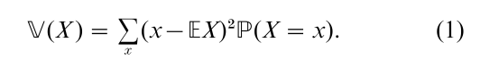
The possible outcomes of the toss of a coin and its respective probabilities can be represented by a random variable. A random variable X is characterized by a set S of possible outcomes and the probability distribution or law of these outcomes: for each x in S, P (X = x) denotes the probability that the outcome results x. In coin-toss the set S is either {head, tail} or {0, 1} and the distribution is given by P (X = 0) = P (X = 1) = 1/2. The mean or expected value E(X ) of a random variable X is the sum of the possible outcomes multiplied by the probability of the outcome: E(X ) = ∑_xx P(X = x). The variance V(X ) describes the square dispersion of the variable around the mean:

A process is a family of random variables labeled by some set. Independent random variables are characterized by the fact that the outcome of one variable does not change the law of the others. For example, the random variables describing the outcomes of different coins are independent. The random variables describing the parity and the value of the face of a dice are not independent: if one knows that the parity is even, then the face can only be 2, 4, or 6.

1.1 Law Of Large Numbers And Central Limit Theorem

A sequence of independent random variables is the most unpredictable probabilistic object. However, questions involving a large number of variables get almost deterministic answers. Consider a sequence of independent and identically distributed random variables X₁, X₂,… with common mean µ and finite variance σ². The partial sums of the first n variables is defined by S_n = X₁ + … + X_n and the empiric mean of the first n outcomes by S_n/n. The expectation and the variance of S_n are given by E(S_n) = nµ and V(S_n) = nσ². The law of large numbers says that as n increases, the random variable S_n/n is very close to µ. More rigorously, for any value ε > 0, the probability that S_n/n differs from its expectation by more than ε can be made arbitrarily close to zero by making n sufficiently large.

The Central Limit Theorem says that the distance between S_n and nµ is of the order √n. More precisely it gives the asymptotic law of the difference when n goes to ∞:

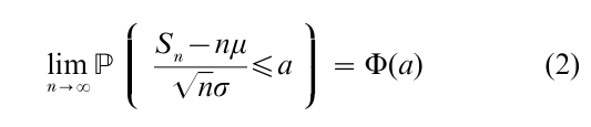
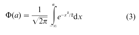
where Φ is the normal cumulative distribution function defined by

1.2 Law Of Small Numbers And Poisson Processes

Consider a positive real number λ and a double labeled sequence X(i, n) of variables with law [X(i, n) = 1] = λ/n, P[X(i, n) = 0] = 1 – λ/n; n is a natural number, that is, in the set {0, 1,…} and i is in the ‘shrinked’ lattice {1/n, 2/n,…} the nomenclature comes from the fact that as n grows the distance between points diminishes). In this way, for fixed n there are around n random variables sitting in each interval of length one but each variable X(i, n) has a small probability of being 1 and a large probability of being 0 in such a way that the mean number of ones in the interval is around λ for all n. When n goes to infinity the above process converges to a Poisson process. This process is characterized by the fact that the number N(Λ) of ones in any interval Λ is a Poisson random variable with mean λm(Λ), where m(Λ) = length of Λ:P[N(Λ) = k] = e^−λm(Λ)[λm(Λ)]^k /k!; furthermore, the numbers of ones in disjoint regions are independent. A bi-dimensional lattice consists of points with two coordinates i = (i₁, i₂) with both i₁ and i₂ natural numbers and analogously the points in a d-dimensional lattice have d coordinates. When i runs in a multidimensional shrinked lattice, the limit is a multidimensional Poisson process. This is called the law of small numbers.

The one-dimensional Poisson process has the property that the distances between successive ones are independent random variables with exponential distribution (it is said that T has exponential distribution with parameter λ if P(T > t) = ^e-λt). In this paper, one-dimensional Poisson process will be called a Poisson clock and the times of occurrence of ones will be called rings.

The classic book for coin-tossing and introductory probability models is Feller (1971). Modern approaches include Fristedt and Gray (1997), Bremaud (1999) and Durrett (1999a). Aldous (1989) describes how the Poisson process appears as the limit of many distinct phenomena.

2. Static Models

2.1 Percolation

Suppose that each site of the two-dimensional lattice is painted black with probability p and white with probability 1 – p independent of the other sites. There is a black path between two sites if it is possible to go from one site to the other jumping one unity at each step and always jumping on black sites. The cluster of a given site x is the set of (black) sites that can be attained following black paths started at x. Of course, when p is zero the cluster of the origin is empty and when p is one, it is the whole lattice. The basic question is about the size of the cluster containing the origin. When this size is infinity, it is said that there is percolation. It has been proven that there exists a critical value p_c such that when p is smaller than or equal to p_c there is no percolation, and when p is bigger than p_c there is percolation with positive probability. This is the typical situation of phase transition: a family of models depending on a continuous parameter which show a qualitative change of behavior as a consequence of a small quantitative change of the parameter. Oriented percolation occurs when the paths can go from one point to the next following only two directions; for example South–North and West– East. The standard reference for percolation is Grimmett (1999).

2.2 Random Graphs

Consider a set of n points and a positive number c. Then, with probability c/n, connect independently each pair of points in the set. The result is a random graph with some number of connected components. Let L₁(n) be the number of points in the largest connected component. It has been proven that as the number of points n increases to infinity the proportion L₁(n)/n of points in the largest component converges to some value γ and that if c > 1 then γ > 0 and that if c ≤ 1, γ = 0. This means that if the probability of connection is sufficiently large, a fraction of points is in the greatest component. In this case this is called the giant component. The number of points in any other component, when divided by n, always converges to zero; hence there is at most one giant component. The fluctuations of the giant component around γn, the behavior of smaller components, and many other problems of random graph theory can be found in Bollobas (1998).

3. Marko Chains

A Markov chain is a process defined iteratively. The ingredients are a finite or countable state space S, a sequence of independent random variables U_n uniformly distributed in the interval [0, 1], and a transition function F which to each state x and number u in the unit interval assigns a state y = F(x, u). The initial state X₀ is either fixed or random and the successive states of the chain are defined iteratively by X_n = F(X_n−1, U_n). That is, the value of the process X_n at each step n is a function of the value X_n−1 at the preceding step and of the value of a uniform random variable U_n independent of everything. In this sense a Markov chain has no memory. The future behavior of the chain given the present position does not depend on how this position was attained. Let Q(x, y) = P(F(x, U_n) = y), the probability that the chain at step n be at state y given that it is at state x at time n – 1. Since this probability does not depend on n the chain is said to be homogeneous in time. The transition matrix Q is the matrix with entries Q(x, y).

When it is possible to go from any state to any other the chain is called irreducible, otherwise reducible. The state space of reducible chains can be partitioned in subspaces in such a way that the chain is irreducible in each part. Irreducible chains in finite state spaces stabilize in the sense that the probability of finding the chain at each state converges to a probability distribution π that satisfies the balance equations: π( y) = ∑_xπ(x)Q(x, y). The measure π is called invariant for Q because if the initial state X₀ has law π then the law of X_n will be π for all future time n. When there is a unique invariant measure π the proportion of time the chain spends in any given state x converges to π(x) when time goes to infinity no matter how the initial state is chosen. This is a law of large numbers for Markov chains. The expected time the chain needs to come back to x when starting at x at time zero is 1/π(x). When the state space has a countable (infinite) number of points it is possible that there is no invariant measure; in this case the probability of finding the chain at any given state goes to zero; that is, the chain ‘drives away’ from any fixed finite region. It is possible also to define Markov chains in noncountable state spaces, but this will not be discussed here.

3.1 Coupling

Two or more Markov chains can be constructed with the same uniform random variables Un. This is called a coupling and it is one of the major tools in stochastic processes. Applications of coupling include proofs of convergence of a Markov chain to its invariant measure, comparisons between chains to obtain properties of one of them in function of the other, and simulation of measures that are invariant for Markov chains.

Recent books on Markov chains include Chen (1992), Bianc and Durrett (1995), Fristedt and Gray (1997), Bremaud (1999), Durrett (1999a), Schinazi (1999), Thorisson (2000), Haggstrom (2000), and Ferrari and Galves (2000).

3.2 Examples: Birth–Death And Branching Processes

The state space of the birth–death process is the set of natural numbers {0, 1,…}, the probability to jump from x to x +1 is p_x, a number in [0, 1] and the probability to jump from x to x – 1 is 1 – p_x. It is assumed that p₀ = 1, that is, the process is reflected at the origin. The transition function is given by F(x, u) = x + H(x, u), with H(x, u) = 1 if u < p_x and H(x, u) = -1 if u ≥ p_x. It is possible to find explicit conditions on p_x that guarantee the existence of an invariant measure. For instance, if p_x < a for all x for some a < 1/2, then there exists an invariant measure π. The reason is that the chain has a drift towards the origin where it is reflected. On the other hand, if the drift towards the origin is not sufficiently strong, the chain may have no invariant measure.

The (n + 1)th generation of a branching process consists of the daughters of the individuals alive in the nth generation:

where Z_n is the total number of individuals in the nth generation and X_n,i is the number of daughters of ith individual of the nth generation. Z₀ = 1 and X_n,i are assumed independent and identically distributed random variables with values in {0, 1, 2,…}. When X_n,i = 0 the corresponding individual died without a progeny. The process so defined is a Markov chain in {0, 1, 2,…}; the corresponding transition function F can be easily computed from the distribution of X_n,i. The mean number of daughters of the typical individual µ = EX_n,i (a value that does not depend on n, i) is the crucial parameter to establish the behavior of the process. When µ > 1 the probability that at all times there are alive individuals is positive; in this case the process is called supercritical and in case of survival the number of individuals increases geometrically with n. When µ ≤ 1 the process dies out with probability one (subcritical case). Guttorp (1991) discusses branching processes and their statistics.

4. Interacting Particle Systems

Processes with many interacting components are called interacting particle systems. Each component has state space S and X_t(i) denotes the state of component i at time t; t may be discrete or continuous, generally i belongs to a d-dimensional lattice. The update law of each component typically depends on the state of the other components; this dependence is in general ‘local,’ that is, determined only by the configuration of a few other neighboring components. The references for interacting particle systems are Liggett (1985) and (1999), Durrett (1988) and (1999b), Chen (1992), Schinazi (1999), Fristedt and Gray (1997).

4.1 The Exclusion Process

In this process i belongs to the d-dimensional lattice and X_t(i) assumes only the value 0 and 1. If Xt(i) 0, site i is empty at time t and if X_t(i) = 1, site i is occupied by a particle at time t. The process evolves as follows. Independent Poisson clocks are attached to the sites; when the clock rings at site i (at most one clock rings at any given time), if there is a particle at i, then a site j is chosen at random and the particle tries to jump to j. If j is empty then the particle jumps; if j is already occupied the jump is suppressed. The interaction between particles is embedded in the law of the jump. The simplest case is when the distribution of the jump does not depend on the configuration. In this case the interaction is just reduced to the suppression of jumps attempted to occupied sites and the motion is called the simple exclusion process.

The measure obtained when a particle is put at each site with probability ρ independently of the other sites is called a product measure. A surprising feature of the simple exclusion process with spatially homogeneous jump laws is that if the initial configuration is chosen according to a product measure, then the configuration at any future time will also be distributed with this measure. In other words, product measures are time invariant for the process. Due to the conservative character of the dynamics, i.e., the initial density is conserved, the process accepts a family of invariant measures; there is one invariant product measure for each density ρ in [0, 1].

The main questions are related to the asymptotic behavior of the process when time runs. In many cases it has been proven that the process starting with an initial configuration having an asymptotic density converges as time goes to infinity to the product measure with that density. More detailed questions are related to hydrodynamic limits obtained when large space regions are observed at long times. A particularly interesting case is the symmetric simple exclusion process, for which jumps of sizes y and -y have the same probability. The large space, long time behavior of the symmetric simple exclusion process is governed by the heat equation. For example, in the one-dimensional case it has been proven that the number of particles in the region [aN, bN] at time tN² divided by N converges to∫^b_au(r, t) dr, where u(r, t) is the solution of the heat equation

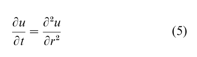
with initial condition u(r, 0) (the initial particle distribution must be related with this condition in an appropriate sense). This is called a law of large numbers or hydrodynamic limit. The limiting partial differential equation represents the macroscopic behavior while the particle system catches the microscopic behavior of the system. The law of the configuration of the process in sites around rN at time tN² converges as N goes to infinity to the product measure with density given by the macroscopic density u(r, t). This is the most disordered state (or measure). This is called propagation of chaos.

When the motion is not symmetric the behavior changes dramatically. The simplest case is the totally asymmetric one-dimensional nearest neighbor simple exclusion process. The particles jump in the one-dimensional integer lattice {… , -1, 0, 1, …}. When the Poisson clock rings at site i, if there is a particle at that site and no particle at i + 1, then the particle jumps to i 1; otherwise nothing changes. To perform the hydrodynamic limit time and space are rescaled in the same way: the number of particles in the region [aN, bN] divided by N at time tN converges to ∫^b_a u(r, t) dt, the solution of the Burgers equation

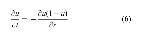
with initial condition u(r, 0). Similar equations can be obtained in the d-dimensional case. Propagation of chaos is also present in this case. Contrary to what happens in the symmetric case, the Burgers equation develops noncontinuous solutions. In particular, consider ρ < λ and the initial condition u(r, 0) equal to ρ if r < 0 and to λ otherwise. Then the solution u(r, t) is ρ if r < (1 – ρ – λ)t and λ otherwise. The well-known phenomenon of highways occur here: the space is divided in two regions sharply separated; one region of low density and high velocity and the other region of high density and low velocity. This phenomenon that was first observed for the Burgers equation (Evans (1998)) was then proven to hold for the microscopic system for the nearest neighbor case. The location of the shock is identified by a perturbation of the system: start with a configuration η coming from a product shock measure, that is, the probability of having a particle at site i is ρ if i is negative and λ if i is positive, and put a particle at the origin. Consider another configuration η´ that coincides with η at all sites but at the origin. η´ is a perturbation of η. Realizing two processes starting with η and η´ respectively, using the same Poisson clocks, there will be only one difference between the two configurations at any given future time. The configuration as seen from the position of this perturbation is distributed approximately as η, that is, with a shock measure. The perturbation behaves as a second class particle; the sites that are occupied by particles of both η and η´ are said to be ‘occupied by a first class particle,’ while the site where η differs from η´ is said to be ‘occupied by a second class particle.’ Following the Poisson clocks, the second class particle jumps backwards when a first class particle jumps over its site and jumps forwards if the destination site is empty. See Liggett (1999).

Special interest has been devoted to the process when the initial condition is ‘there are particles in all negative sites and no particles in the other sites.’ The solution u(r, t) of the Burgers equation with this initial condition is a rarefaction front: u(r, t) is one up to -t, zero from t on and interpolates linearly between 0 and 1 in the interval [-t, t]. This particular case has been recently related to models coming from other areas of applied probability. In particular with increasing subsequences in random permutations, random matrices, last passage percolation, random domino tilings and systems of queues.

Hydrodynamics of particle systems is discussed by Spohn (1991), De Masi and Presutti (1991), and Kipnis and Landim (1999).

4.2 Voter Model

In the voter model each site of a d-dimensional integer lattice (this is the set of d-uples of values in the integer lattice {…, -1, 0, 1,…}) is occupied by a voter having two possible opinions: 0 and 1. At the rings of a Poisson clock each voter chooses a neighbor at random and assumes its opinion. The voter model has two trivial invariant measures: ‘all zeros’ and ‘all ones.’ Of course, if at time zero all voters have opinion zero, then at all future times they will be zero; the same occurs if all voters have opinion one at time zero. Are there other invariant measures? The answer is no for dimensions d = 1 and d = 2 and yes for dimension d ≥ 3. The proof of this result is based on a dual process. This process arises when looking at the opinion of a voter i at some time t. It suffices to go back in time to find the voter at time zero that originates the opinion of i at time t. The space–time backwards paths for two voters may coalesce. In this case the two voters will have the same opinion at that time. The backwards paths are simple random walks. In one or two dimensions, nearest-neighbors random walks always coalesce, while in dimensions greater than or equal to three there is a positive probability that the walks do not coalesce. Hence there are invariant states in three or more dimensions for which different opinions may coexist.

A generalization of the voter model is the random average process. Each voter may have opinions corresponding to real numbers and, instead of looking at only one neighbor, at Poisson rings voters update their opinion with a randomly weighted average of the opinions of the neighbors and adopt it. As in the two-opinions voter model, flat configurations are invariant, but if the system starts with a tilted configuration (for example, voter i has opinion λ_i for some parameter λ ≠ 0), then the opinions evolve randomly with time. It is possible to relate the variance of the opinion of a given voter to the total amount of time spent at the origin by a symmetric random walk. This shows that the variance of the opinion of a given voter at time t is of the order of t in dimension one, log t in dimension 2, and constant in dimensions greater than or equal to 3. The random average process is a particular case of the linear processes studied in Liggett (1985).

5. Future Directions

At the start of the twenty-first century, additional developments for the exclusion process include the behavior of a tagged particle, the convergence to the invariant measure for the process in finite regions, and more refined relations between the microscopic and macroscopic counterpart. The voter model described here is ‘linear’ in the sense that the probability of changing opinion is proportional to the number of neighbors with the opposite opinion. Other rules lead to ‘nonlinear’ voter models that show more complicated behavior. See Liggett (1999). The rescaling of the random average process may give rise to nontrivial limits; this is a possible line of future development.

The contact process, a continuous-time version of oriented percolation, has not been discussed here. The contact process in a graph instead of a lattice may involve three or more phases (in the examples discussed here there were only two phases). The study of particle systems in graphs is a promising area of research.

An important issue not discussed here is related to Gibbs measures; indeed, phase transition was mathematically discussed first in the context of Gibbs measures. One can think of a Gibbs measure as a perturbation of a product measure: configurations have a weight according to a function called energy. Gibbs measures may describe the state of individuals that have a tendency to agree (or disagree) with their neighbors. Stochastic Ising models are interacting particle systems that have as invariant measures the Gibbs measure related to a ferromagnet. Mixtures of Ising models and exclusion processes give rise to reaction diffusion processes, related via hydrodynamic limit with reaction diffusion equations.

An area with recent important developments is Random tilings, which describes the behavior of the tiles used to cover an area in a random fashion. The main issue is how the shape of the boundary of the region determines the tiling. Dynamics on tilings would show how the boundary information transmits. The rescaling of some tilings results in a continuous process called the mass-less Gaussian field; loosely speaking, a multidimensional generalization of the central limit theorem.

An important area is generally called spatial processes. These processes describe the random location of particles in the d-dimensional real space instead of a lattice. The Poisson process is an example of a spatial process. Analogously to Gibbs measures, other examples can be constructed by giving different weight to configurations according to an energy function. The study of interacting birth and death processes having as invariant measure spatial process is recent and worth to develop. This is related also with the so-called perfect simulation; roughly speaking this means to give a sample of a configuration of a process as a function of the uniform random numbers given by a computer. See, for instance, Haggstrom (2000).

Bibliography:

1. Aldous D 1989 Probability Approximations via the Poisson Clumping Heuristic. Applied Mathematical Sciences, 77. Springer-Verlag, New York
2. Bianc P, Durrett R 1995 Lectures on probability theory. In: Bernard P (ed.) Lectures from the 23rd Saint-Flour Summer School held August 18–September 4, 1993. Lecture Notes in Mathematics, 1608. Springer-Verlag, Berlin
3. Bollobas B 1998 Modern Graph Theory. Graduate Texts in Mathematics, 184. Springer-Verlag, New York
4. Bremaud P 1999 Marko Chains. Gibbs Fields, Monte Carlo Simulation, and Queues. Texts in Applied Mathematics, 31. Springer-Verlag, New York
5. Chen M F 1992 From Marko Chains to Nonequilibrium Particle Systems. World Scientific Publishing, River Edge, NJ
6. De Masi A, Presutti E 1991 Mathematical Methods for Hydrodynamic Limits. Lecture Notes in Mathematics, 1501. Springer-Verlag, Berlin
7. Durrett R 1988 Lecture Notes on Particle Systems and Percolation. Wadsworth & Brooks Cole Advanced Books & Software, Pacific Grove, CA
8. Durrett R 1999a Essentials of Stochastic Processes. Springer Texts in Statistics. Springer-Verlag, New York
9. Durrett R 1999b Stochastic Spatial Models. Probability Theory and Applications (Princeton, NJ, 1996), 5–47, IAS Park City Mathematics Series 6, American Mathematical Society, Providence, RI
10. Evans L C 1998 Partial Differential Equations. American Mathematical Society, Providence, RI
11. Feller W 1971 An Introduction to Probability Theory and its Applications, Vol. II, 2nd edn. Wiley, New York
12. Ferrari P A Galves A 2000 Coupling and Regeneration for Stochastic Processes. Association Venezolana de Matematicas, Merida
13. Fristedt B, Gray L 1997 A Modern Approach to Probability Theory: Probability and its Applications. Birkhauser Boston, Boston, MA
14. Grimmett G 1999 Percolation, 2nd edn. Grundlehren der mathematischen Wissenschaften [Fundamental Principles of Mathematical Sciences], 321. Springer-Verlag, Berlin
15. Guttorp P 1991 Statistical Inference for Branching Processes. Wiley, New York
16. Haggstrom 2000 Finite Marko Chains and Algorithmic Applications. To appear.
17. Kipnis C, Landim C 1999 Scaling Limits of Interacting Particle Systems. Grundlehren der mathematischen Wissenschaften [Fundamental Principles of Mathematical Sciences], 320. Springer-Verlag, Berlin
18. Liggett T M 1985 Interacting Particle Systems. Grundlehren der mathematischen Wissenschaften [Fundamental Principles of Mathematical Science], 276. Springer-Verlag, New York
19. Liggett T M 1999 Stochastic Interacting Systems: Contact, Voter and Exclusion Processes. Grundlehren der mathematischen Wissenschaften [Fundamental Principles of Mathematical Sciences], 324. Springer-Verlag, Berlin
20. Schinazi R B 1999 Classical and Spatial Stochastic Processes. Birkhauser Boston, Boston, MA
21. Spohn H 1991 Large Scale Dynamics of Interacting Particles. Springer-Verlag, Berlin
22. Thorisson H 2000 Coupling, Stationarity, and Regeneration: Probability and its Applications. Springer-Verlag, New York