Survival Analysis Research Paper

A cohort study involves selecting a representative set of individuals from some target population and following those individuals forward in time in order to record the occurrence and timing of the failures. Often, some study subjects will still be without failure at the time of data analysis, in which case their failure times T will be known only to exceed their corresponding censoring times. In this case, the censoring time is defined as the time elapsed from the origin to the latest follow-up time, and the failure time is said to be right censored. Right censorship may also arise because subjects drop out the study, or are lost to follow-up. A key assumption underlying most survival analysis methods is that the probability of censoring an individual at a given follow-up time does not depend on subsequent failure times. This independence assumption implies that individuals who are under study at time t are representative of the cohort and precludes, for example, the censoring of individuals at time t because, among individuals under study at that time, they appear to be at unusually high (or low) risk of failure. (This assumption can be relaxed to independence between censoring and failure times conditional on the preceding histories of covariates.) The reasonableness of the independent censoring assumption, which usually cannot be tested directly, should be considered carefully in specific applications.

The distribution of a failure time variate T > 0 is readily represented by its survivor function F (t) = P(T > t). If T is absolutely continuous, its distribution can also be represented by the probability density function f (t) = – dF (t)/dt or by the hazard, or instantaneous failure rate, function defined by

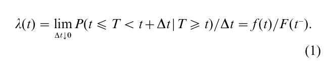
Note that

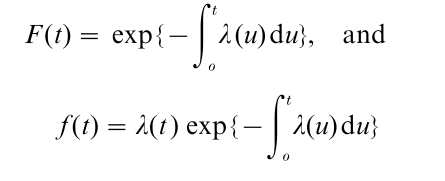
for 0 < t < ∞

In a similar way, the distribution of a discrete failure time variate T, taking values on x₁ < x₂ < …, can be represented by its survivor function, its probability function f (x_i) = P(T = x_i), i = 1, 2 … , or its hazard function λ(x_i) = P(T = x_i|T ≥ x_i) = f(x_i)|F(x_i^–). Note that

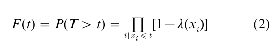
as arises through thinking about the failure mechanism unfolding sequentially in time. To survive past time t where x_j ≤ t < x_j+1, an individual must survive in sequence each of the points x₁,…, x_j with conditional probabilities 1 – λ(x_i), i = 1,…, j.

It is often natural and insightful to focus on the hazard function. For example, human mortality rates are known to be elevated in the first few years of life, to be low and relatively flat for the next three decades or so, and then to increase rapidly in the later decades of life. Similarly, comparison of hazard rates as a function of time from randomization for a new treatment compared with control can provide valuable insights into the nature of treatment effects. Hazard function modeling also integrates nicely with a number of key strategies for selecting study subjects from a target population. For example, if one is studying disease occurrence as it depends upon the age of study subjects, hazard function models readily accommodate varying ages at entry into the study cohort since the conditioning event in (1) specifies that the individual is surviving and event-free at age t. Again one needs to assume that selected subjects have hazard rates that are representative (conditional on covariates) of those at risk for the target population.

2. Estimation And Comparison Of Survival Curves

Suppose that a cohort of individuals has been identified at a time origin t = 0 and followed forward in time. Suppose that failures are observed at times t₁ < t₂ < … < t_k. Just prior to the failures observed at time t_j, there will be some number, r_j, of cohort members that are under active follow-up. That is, the failure and censoring times for these r_j members occur at time t_j or later. Of these r_j individuals, some number, d_j, are observed to fail at t_j. The empirical failure rate or estimated hazard at t_j is then d_j /r_j, and the empirical survival rate is (1 – d_j/r_j). The empirical failure rate at all times other than t₁,…, t_k in the follow-up period is zero. The Kaplan and Meier (1958) estimator of the survivor function F at follow-up time t is

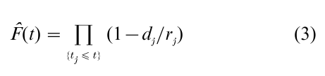
the product of the empirical survivor rates across the observed failure times less than or equal to t. Note that F estimates the underlying survivor function F at those times where there are cohort members at risk. For (3) to be valid, the cohort members at risk at any follow-up time t must have the same failure rate operating as does the target population at that follow-up time. Thus, the aforementioned independent censoring assumptions are needed.

The hazard rate estimators d_j/r_j, j = 1,…, k can be shown to be uncorrelated, giving rise to the Green- wood variance estimator

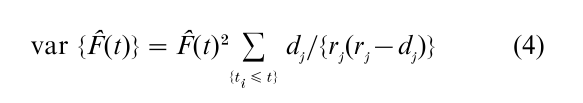
for F(t). In order to show asymptotic results for the estimator F(t), for example that F(t) is a consistent estimator of F(t), it is necessary to restrict the estimation to a follow-up interval [0, τ) within which the size of the risk set (i.e., number of individuals under active follow-up) becomes large as the sample size (n) increases. Under these conditions, n^1/2 {F(t) – F(t)}; 0 ≤ t < τ can be shown to converge weakly to a mean-zero Gaussian process, permitting the calculation of approximate confidence intervals and bands for F on [0, τ). Applying the asymptotic results to the estimation of log {–log F(t)}, which has no range restrictions, is suggested as a way to improve the coverage rates of asymptotic confidence intervals and bands (Kalbfleisch and Prentice 1980, pp. 14, 15).

Consider a test of equality of m survivor functions F₁, … , F_m on the basis of failure-time data from each of m populations. Let t₁ < t₂ < … < t_k denote the ordered failure times from the pooled data, and again let d_j failures occur out of the r_j individuals at risk just prior to time t_j, j = 1,…, k. Also, for each sample i = 1,…, m, let d_ij denote the number of failures at t_j, and r_ij denote the number at risk at t_j⁻. Under the null hypothesis F₁ = F₂ = … = F_m the conditional distribution of d_1j,…, d_mj given (d_j, r_1j,…, r_mj) is hyper-geometric from which the conditional mean and variance of d_ij are respectively u_ij = r_ij(d_j/r_j) and (V_j)_ii = r_ij(r_i – r_ij)d_j(r_j – d_j)r_j⁻²(r_j – 1)⁻¹. The conditional covariance of d_ij and d_1j is

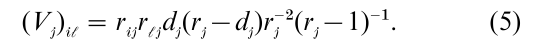
Hence the statistic vj = (d_1j – u_1j,…, d_mj – u­) has conditional mean zero and variance Vj under the null hypothesis. The summation of these differences across failure times,

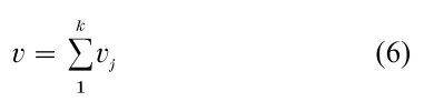
is known as the logrank statistic (Mantel 1966, Peto and Peto 1972). The contributions to this statistic across the various failure times are uncorrelated, and v´V⁻¹v generally has an asymptotic chi-square distribution with m 1 degrees of freedom where V = ∑^k₁V_j and a ‘prime’ denotes vector transpose.

This construction also shows that a broad class of ‘censored data rank tests’ of the form ∑^k₁w_j v_j also provide valid tests of the equality of the m survival curves. In these tests, the ‘weight’ w_j at time t_j can be chosen to depend on the above conditioning event at t_j, or on data collected before t_j, more generally. The null hypothesis variancek o f these test statistics is readily estimated by ∑^k₁w²_j V_j, again leading to an asymptotic chi-square (m – 1) test statistic. The special case w_j = F(t_j⁻) generalizes the Wilcoxon rank sum test to censored data in a natural fashion (e.g., Peto and Peto 1972, Prentice 1978) and provides an alternative to the logrank test that assigns greater weight to earlier failure times. More adaptive tests can also be entertained (e.g., Harrington and Fleming 1982).

3. Failure-Time Regression: The Cox Model

3.1 Model Development

The same type of conditional probability argument generalizes to produce a flexible and powerful regression method for the analysis of failure-time data. This method was proposed in the fundamental paper by Cox (1972) and is referred to as Cox regression or as relative risk regression.

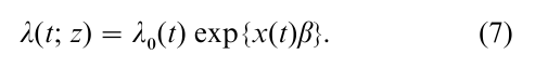
Suppose that each subject has an associated vector of covariates z´ = (z₁, z₂,…). For example, the elements of z may include primary exposure variables and confounding factor measurements in an epidemiologic cohort study, or treatment indicators and patient characteristics in a randomized clinical trial. Let λ(t; z) denote the hazard rate at time t for an absolutely continuous failure time T on an individual with covariate vector z. Now one requires the censoring patterns, and the cohort entry patterns, to be such that the hazard rate λ(t; z) applies to the cohort members at risk at follow-up time t and covariate value z for each t and z. The Cox regression model specifies a parametric form for the hazard rate ratio λ(t; z)/λ(t; z₀), where z₀ is a reference value (e.g., z₀ = 0). Because this ratio is nonnegative, it is common to use an exponential parametric model of the form exp {x(t)β}. The vector x(t) = {x₁(t),…, x_p(t)} includes derived covariates that are functions of the elements of z (e.g., main effects and interactions) and possibly product (interaction) terms between z and t. The vector β´ = (β₁,…, β_p) is a p-vector of regression parameters to be estimated. Denoting λ₀(t) = λ(t; z₀) allows the model to be written in the standard form

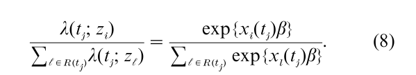
As in previous section let t₁ < t₂ < … < t_k denote the ordered distinct failure times observed in follow-up of the cohort, and let d_j denote the number of failures at t_j. Also let R(t_j) denote the set of labels of individuals at risk for failure at t_j⁻. We suppose first that there are no ties in the data so that d_j = 1. The conditional probability that the ith individual in the risk set with covariate z_i fails at t_j, given that d_j = 1 and the failure, censoring (and covariate) information prior to t_j, is simply

The product of such terms across the distinct failure times

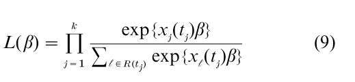
is known as the partial likelihood function for the relative risk parameter β.

If one denotes L( β) = ∏^k_j=1 L_j( β), then the fact that the scores log L_j( β)/ϐβ, j = 1,…, k have mean zero and are uncorrelated (Cox 1975) suggests that, under regularity conditions, the partial likelihood (9) has the same asymptotic properties as does the usual likelihood function. Let β denote the maximum partial likelihood estimate that solves ϐ log L( β) / ϐβ = 0. Then, n^1/2( β – β) will generally converge, as the sample size n becomes large, to a p-variate norma1 distribution having mean zero and covariance matrix consistently estimated by n^-1ϐ² log L( β)/ϐβϐβ´. This result provides the usual basis for tests and confidence intervals on the elements of β.

Even though we are working with continuous models, there will often be some tied failure times. If the ties are numerous, it may be better to model the data using a discrete failure-time model. Often, however, a simple modification to (9) is appropriate. When the d_j are small compared with the r_j, the approximate partial likelihood (Peto and Peto 1972, Breslow 1974)

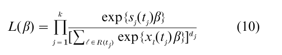
is quite adequate for inference, where s_j(t_j) = ∑_iϵDxi(tj) and D_j represents the set of labels of individuals failing at t_j. Efron (1977) suggested an alternate approximation that is only slightly more complicated and is somewhat better. Both the Breslow and Efron approximations are available in software packages.

3.2 Special Cases And Generalizations

Some special cases of the modeled regression vector x(t) illustrate the flexibility of the relative risk model (7). If one restricts x(t) = x, to be independent of t, then the hazard ratios at any pair of z-values are constant. This gives the important proportional hazards special case of (7). For example, if the elements of z include indicator variables for m – 1 of m samples and x(t) = (z₁,…, z_m−1) then each e^βj, j = 1,…, m – 1 denotes the hazard ratio for the jth sample compared with the last (mth) sample. In this circumstance the score test for β = 0 arising from (9) reduces to the logrank test of the preceding section.

The constant hazard ratio assumption, in this example, can be relaxed by defining x(t) = {g(t)z₁,…, g(t)z_m−1} for some specified function g of follow-up time. For example g(t) = log t would allow hazard ratios of the form t^βj for the jth sample compared with the mth. This gives a model in which hazard ratio for the jth vs. the mth population increase (β_j > 0) or decrease (β_j < 0) monotonely from unity as t increases. The corresponding score test would be a weighted logrank test for the global null hypothesis. More generally one could define x(t) = {z₁,…, z_m−1, g(t)z₁,…, g(t)z_m−1}. This model is hierarchical with main effects for the sample indicators and interactions with g(t). A test that the interaction coefficients are zero provides an approach to checking for proportionality of the hazard functions. Departure from proportionality would imply the need to retain some product terms in the model, or to relax the proportionality assumption in some other way.

As a second special case consider a single quantitative predictor variable z. Under a proportional hazards assumption one can include various functions of z in the modeled (time independent) regression vector x(t) = x for model building and checking, just as in ordinary linear regression. The proportionality assumption can be relaxed in various ways including setting x(t) = {xI₁(t),…, xI_q(t)} where I₁(t),…, I_q(t) are indicator variables for a partition of the study follow-up period. The resulting model allows the relative risk parameters corresponding to the elements of x = x(z) to be separately estimated in each follow-up interval. This provides a means for testing the proportionality assumption, and relaxing it as necessary to provide an adequate representation of the data.

The above description of the Cox model (7) assumed that a fixed regression vector z was measured on each study subject. It is important to note that (7) can be relaxed to include measurements of stochastic covariates that evolve over time. This does not complicate the development of (9) or (10). Specifically, if z(t) denotes a study subject’s covariates at follow-up time t, and Z(t) = {z(u); u < t} denotes the corresponding covariate history up to time t, then the hazard rate λ(t; Z(t)} can be modeled according to the right side of (7) with x(t), comprising functions of Z(t) and product terms between such functions and time.

Careful thought must be given to relative risk parameter interpretation in the presence of stochastic covariates. For example, the interpretation of treatment effect parameters in a randomized controlled trial may be affected substantially by the inclusion of postrandomization covariates when those covariates are affected by the treatment. However, careful use of such covariates can serve to identify mechanisms by which the treatment works.

3.3 Survivor Function Estimation

The cumulative ‘baseline’ hazard function Λ₀(t) = ∫^t₀ λ₀(u)du (7) can be simply estimated (Breslow 1974) by

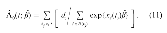
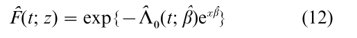
If x(t) = x is time-independent, the survivor function F(t; z) = p{T > t|z} = exp{ -Λ₀(t)e^xβ} is estimated by

A slightly more complicated estimator F(t; z) is available if x is time-dependent.

A practically important generalization of (7) allows the baseline hazard to depend on strata s = s(z), or more generally s = s(z, t) so that

where s takes integer values 1, 2,…, m indexing the strata. This provides another avenue for relaxing a proportional hazards assumption. The stratified partial likelihood is simply a product of terms (9) over the various strata.

3.4 Asymptotic Distribution Theory

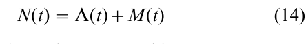
The score function U( β) = ϐlog L( β)/ ϐβ from (9) involves a sum of terms that are uncorrelated but not independent. The theory of counting processes and martingales provides a framework in which this uncorrelated structure can be described, and a formal development of asymptotic distribution theory. Specifically, the counting process N for a study subject is defined by N(t) = 0 prior to the time of an observed failure, and N(t) = 1 at or beyond the subject’s observed failure time. The counting process can be decomposed as

where, under independent censorship,

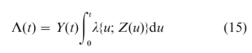
and M(t) is a locally square integrable martingale. Note that in the ‘compensator’ Λ the ‘at risk’ process Y is defined by Y(t) = 1 up to the time of failure or censoring for the subject and zero thereafter. The decomposition (14) allows the logarithm of (9), and its derivatives, and the cumulative hazard estimator (11), to be expressed as stochastic integrals with respect to martingales, to which powerful convergence theorems apply. Anderson and Gill (1982) provide a thorough development of asymptotic distribution theory for the Cox model using these counting process techniques, and provide weak conditions for the joint asymptotic convergence of n^1/2 ( β – β) and to Λ₀( , β) to Gaussian processes. The books by Fleming and Harrington (1991) and Andersen et al. (1993) use the counting process formulation for the theory of each of the statistics mentioned above, and for various other tests and estimators.

4. Other Failure-Time Regression Models

4.1 Parametric Models

Parametric failure-time regression models may be considered as an alternative to the semiparametric Cox model (7). For example, requiring λ (t) in (7) to be a constant or a power function of time gives exponential and Weibull regression models respectively. The maximum partial likelihood estimate β of the preceding section is known to be fully efficient within the semiparametric model with λ₀(t) in (7) completely unspecified. While some efficiency gain in β estimation is possible if an assumed parametric model is true, such improvement is typically small and may be more than offset by a lack of robustness.

Of course there are many parametric regression models that are not contained in the Cox model (7). One such class specifies a linear model for the logarithm of time to failure,

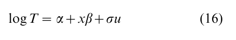
where x = x(z) is comprised of functions of a fixed regression vector z. The parameters α and σ are location and scale parameters, β is a vector of regression parameters and u is an error variate. Because regression effects are additive on log T, or multiplicative on T, this class of models is often referred to as the accelerated failure-time model. If the error u has an extreme value distribution with density f(u) = exp (u –e^u), then the resulting model for T is the Weibull regression model previously mentioned. More generally, any specified density for u induces a hazard function model λ(t; z) for T to which standard likelihood estimation procedures apply, and asymptotic distribution theory can be developed based again on counting process theory.

4.2 A Competing Semiparametric Model

The model (16) has also been studied as a semiparametric class in which the distribution of the error u is unspecified. Prentice (1978) considered the likelihood for the censored data rank vector based on the ‘residuals’ v( β₀) = log T – xβ₀ to generate a linear rank statistic

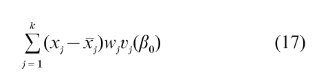
for testing β = β₀. In (l7), v_j( β₀) is the jth largest of the uncensored v(β₀) values, x_j is the corresponding modeled covariate value, x_j is the average of the x-values for the individuals having ‘residual’ equal or greater than v_j( β₀), and w_j is a weight, usually taken to be identically equal to one (logrank scores). An estimator of β of β in (17) can be defined as a value of β₀ for which the length of the vector (17) is minimized. The calculation of β is complicated by the fact that (17) is a step function that requires a reranking of the residuals at each trial value of β₀. However, simulated annealing methods have been developed (Lin and Geyer 1992) for this calculation, and resampling methods have been proposed for the estimation of confidence intervals for the elements of β (Parzen et al, 1994). See Ying (1993) for an account of the asymptotic theory for β.

The model (16) implies a hazard function of the form

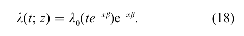
This form suggests a time-dependent covariate version of the accelerated failure-time model (e.g., Cox and Oakes 1984, Robins and Tsiatis 1992) given by

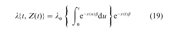
which retains the notion of the preceding covariate history implying a rescaling or acceleration, by a factor e^−x(t)β, of the rate at which a study subject traverses the failure-time axis.

5. Multiple Failure Times And Types

5.1 Multiple Failure Types And Competing Risks

Suppose that individuals are followed for the occurrence of a univariate failure time, but that the failure may be one of several types. The type i specific hazard function at follow-up time t, for an individual having preceding covariate Z(t) can, for example, be specified as

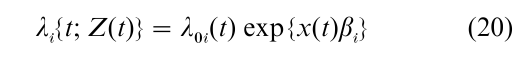
where λ₀ i is a baseline hazard for the ith failure type and β_i is a corresponding relative risk parameter. Estimation of β₁, β₂,…, under independent censorship is readily based on a partial likelihood function that is simply a product of terms (9) over distinct failure types (e.g., Kalbfleisch and Prentice 1980, Chap. 7). In fact, inference on a particular regression vector β_i and corresponding cumulative hazard function Λ_0i is based on (9) upon censoring the failures of types other than (i) at their observed failure times. Accelerated failure time regression methods similarly generalize for the estimation of type-specific regression parameters.

Very often questions are posed that relate to the relationship between the various types of failure. It should be stressed that data on failure time and failure type alone are insufficient for studying the interrelation among the failure mechanisms for the different types, rather one generally requires the ability to observe the times of multiple failures on specific study subjects.

5.2 Recurrent Events

Suppose that there is a single type of failure, but that individual study subjects may experience multiple failures over time. Examples include multiple disease recurrences among cancer patients, multiple job losses in an employment history study, or multiple breakdowns of a manufactured item. The counting process N at follow-up time t is defined as the number of failures observed to occur on the interval (0, t] for the specific individual. The asymptotic theory of Andersen and Gill (1982) embraced such counting processes in which the failure rate at time t was of Cox model form

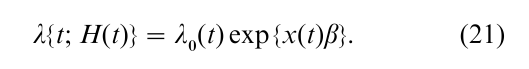
In this expression, the conditioning event H(t) includes the individual’s counting process history, in addition to the corresponding covariate history prior to follow- up time t. Hence the modeled covariate x(t) must specify the dependence of the failure rate at time t both on the covariates and on the effects of the individual’s preceding failure history. Various generalizations of (21) may be considered to acknowledge these conditioning histories in a flexible fashion. For example, λ₀ can be stratified on the number of preceding failures on the study subject; or the argument in λ₀ may be replaced by the gap time from the preceding failure (Prentice et al 1981).

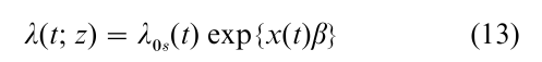
A useful alternative to (21) involves modeling a marginalized failure rate in which one ‘forgets’ some aspects of H(t). For example, one could replace H(t) in (21) by the covariate history Z(t) and the number s = s(t) of failures for the individual prior to time t. A Cox-type model λ₀s(t) exp {x(t) β_s } for the resulting failure rate function would allow one to focus on covariate effects without having to model the timing of the s preceding failures. While the parameters βs can again be estimated using the score equations from a stratified version of (9) a corresponding sandwich variance formula is needed to acknowledge the variability introduced by the nonincreasing conditioning event (Wei et al. 1989, Pepe and Cai 1993, Lawless and Nadeau 1995).

5.3 Correlated Failure Times

In some settings, such as group randomized intervention trials, the failure times on individuals within groups may be correlated, a feature that needs to be properly accommodated in data analysis. In other contexts, such as family studies of disease occurrence in genetic epidemiology, study of the nature of the dependency between failure times may be a key research goal.

In the former situation, hazard-function models of the types described above can be specified for the marginal distributions of each of the correlated failure times, and marginal regression parameters may be estimated using the techniques of the preceding sections. A sandwich-type variance estimator is needed to accommodate the dependencies between the estimating function contributions for individuals in the same group (Wei et al 1989, Prentice and Hsu 1997).

If the nature of the dependence between failure times is of substantive interest it is natural to consider nonparametric estimation of the bivariate survivor function F(t₁, t₂) = p(T₁ > t₁, T₂ > t₂). Strongly consistent and asymptotically Gaussian nonparametric estimators are available (Dabrowska 1988, Prentice and Cai 1992), though these estimators are nonparametric efficient only if T₁ and T₂ are independent (Gill et al. 1995). Nonparametric efficient estimators away from this independence special case can be developed through a grouped data nonparametric maximum likelihood approach (Van der Laan 1996), though this estimation problem remains an active area of investigation.

5.4 Frailty Models

There is also substantial literature on the use of latent variables for the modeling of multivariate failure times. In these models, failure times are assumed to be independent given the value of a random effect, or frailty, which is usually assumed to affect the hazard function in a multiplicative (time-independent) fashion.

One of the simplest such models arises if a frailty variate has a gamma distribution. This generates the Clayton (1978) bivariate model with joint survivor function

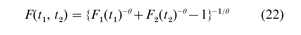
where θ controls the extent of dependence between T₁ and T₂ with maximal positive dependence as θ → ∞, maximal negative dependence as θ → -1, and independence at θ = 0 (e.g., Oakes 1989).

Nielsen et al. (1992) generalize this model to include regression variables and propose an expectationmaximization algorithm with profiling on θ for model fitting. Andersen et al. (1993) and Hougaard (2000) provide fuller accounts of this approach to multivariate failure-time analysis.

6. Additional Survival Analysis Topics

Space permits only brief mention of a few additional survival analysis topics: Considerable effort has been devoted to model building and testing aspects of the use of failure-time regression models. The monograph by Therneau and Grambsch (2000) summarizes much of this work in the context of the Cox model (7).

The cost of assembling covariate histories has led to a number of proposals for sampling within cohorts, whereby the denominator terms in (9) are replaced by suitable estimates, based on a subset of the subjects at risk. These include nested case-control sampling in which the denominator at t_j is replaced by a sum that involves the individual failing at t_j and controls randomly selected from R(t_j), independently at each distinct t_j, and case-cohort sampling in which the denominator summation at t consists of the failing individual along with the at risk members of a fixed random subcohort (see Samuelson (1997) for a recent contribution).

Considerable effort has also been directed to allowing for measurement error in regression variables, particularly in the context of the Cox model (7) with time-independent covariates. Huang and Wang (2000) provide a method for consistently estimating β in (7) under a classical measurement error model, and provide a summary of the literature on this important topic.

Testing and estimation on regression parameters has also been considered in the context of clinical trials under sequential monitoring. The recent book by Jennison and Turnbull (2000) summarizes this work.

Additional perspective on the survival analysis literature can be obtained from the overviews of Anderson and Keiding (1999) and of Oakes (2000). Goldstein and Harrell (1999) provide a description of the capabilities of various statistical software packages for carrying out survival analyses.

Bibliography:

1. Andersen P K, Gill R D 1982 Cox’s regression model for counting processes: A large sample study. Annals of Statistics 10: 1100–20
2. Andersen P K, Borgan O, Gill R D, Keiding N 1993 Statistical Models Based on Counting Processes. Springer, New York
3. Andersen P K, Keiding N 1999 Survival analysis, overview. Encyclopedia of Biostatistics. Armitage P, Colton T (eds.). Wiley, New York, Vol. 6, pp. 4452–61
4. Breslow N E 1974 Covariance analysis of censored survival data. Biometrics 30: 89–99
5. Clayton D 1978 A model for association in bivariate life tables and its application in studies of familial tendency in chronic disease incidence. Biometrika 65: 141–51
6. Cox D R 1972 Regression models and life tables (with discussion). Journal of the Royal Statistical Society, Series B, 34: 187–220
7. Cox D R 1975 Partial likelihood. Biometrika 62: 269–276
8. Cox D R, Oakes D 1984 Analysis of Survival Data. Chapman & Hall, London
9. Dabrowska D 1988 Kaplan-Meier estimate on the plane. Annals of Statistics 16: 1475–89
10. Efron B 1977 Efficiency of Cox’s likelihood function for censored data. Journal of the American Statistical Association 72: 557–65
11. Fleming T R, Harrington D D 1991 Counting Processes and Survival Analysis. Wiley, New York
12. Gill R D, Van der Laan M, Wellner J A 1995 Inefficient estimators of the bivariate survival function for three models. Annals of the Institute Henri Poincare, Probability and Statistics 31: 547–97
13. Goldstein R, Harrell F 1999 Survival analysis, software. Encyclopedia of Biostatistics. Armitage P, Colton T (eds.). Wiley, New York, Vol. 6, pp. 4461–6
14. Harrington D P, Fleming T R 1982 A class of rank test procedures for censored survival data. Biometrika 69: 133–43
15. Hougaard P 2000 Analysis of Multivariate Sur i al Data. Springer, New York
16. Huang Y, Wang C Y 2000 Cox regression with accurate covariates unascertainable: A nonparametric correction approach. Journal of the American Statistical Association 95: 1209–19
17. Jennison C, Turnbull B W 2000 Group Sequential Methods with Application to Clinical Trials. Chapman & Hall, New York
18. Kalbfleisch J D, Prentice R L 1980 The Statistical Analysis of Failure Time Data. Wiley, New York
19. Kaplan E L, Meier P 1958 Nonparametric estimation from incomplete observations. Journal of the American Statistical Association 53: 457–81
20. Lawless J F, Nadeau C 1995 Some simple and robust methods for the analysis of recurrent events. Technometrics 37: 158–68
21. Lin D Y, Geyer C J 1992 Computational methods for semiparametric linear regression with censored data. Journal of Computational and Graphical Statistics 1: 77–90
22. Lin D Y, Wei J L, Ying Z 1998 Accelerated failure time models for counting processes. Biometrika 85: 608–18
23. Mantel N 1966 Evaluation of survival data and two new rank order statistics arising in its consideration. Cancer and Chemotherapy Reports 50: 163–70
24. Nielsen G G, Gill R D, Andersen P K, Sorensen T I A 1992 A counting process approach to maximum likelihood estimation in frailty models. Scand Journal of Statistics 19: 25–43
25. Oakes D 1989 Bivariate survival models induced by frailties. Journal of the American Statistical Association 84: 487–93
26. Oakes D 2000 Survival analysis. Journal of the American Statistical Association 95: 282–5
27. Parzen M I, Wei L J, Ying Z 1994 A resampling method based on pivotal estimating functions. Biometrika 68: 373–9
28. Pepe M S, Cai J 1993 Some graphical displays and marginal regression analysis for recurrent failure times and time dependent covariates. Journal of the American Statistical Association 88: 811–20
29. Peto R, Peto J 1972 Asymptotically efficient rank invariant test procedures (with discussion). Journal of the Royal Statistical Society Series A, 135: 185–206
30. Prentice R L 1978 Linear rank tests with right censored data. Biometrika 65: 167–79
31. Prentice R L, Cai J 1992 Covariance and survivor function estimation using censored multivariate failure time data. Biometrika 79: 495–512
32. Prentice R L, Hsu L 1997 Regression on hazard ratios and cross ratios in multivariate failure time analysis. Biometrika 84: 349–63
33. Prentice R L, Williams B J, Peterson A V 1981 On the regression analysis of multivariate failure time data. Biometrika 68: 373–9
34. Robins J M, Tsiatis A A 1992 Semiparametric estimation of an accelerated failure time model with time-dependent covariates. Biometrika 79: 311–9
35. Samuelsen S O 1997 A pseudolikelihood approach to analysis of nested case-control studies. Biometrika 84: 379–84
36. Therneau T, Grambsch P 2000 Modeling Survival Data: Extending the Cox Model. Springer, New York
37. Van der Laan M J 1996 Efficient estimation in the bivariate censoring model and repairing NPMLE. Annals of Statistics 24: 596–627
38. Wei I J, Lin D Y, Weissfeld L 1989 Regression analysis of multivariate incomplete failure time data by modeling marginal distributions. Journal of American Statistical Association 84: 1065–73
39. Ying Z 1993 A large sample study of rank estimation for censored regression data. Annals of Statistics 21: 76–99