Multivariate Analysis Research Paper

Although there are many practical applications for each of the methods discussed in this overview, we cite some applications for the classification and discrimination methods in Sect. 6.5. The goal is to distinguish between two populations, or to classify a new observation in one of the populations. Examples are (a) solvent and insolvent companies based on several financial measures; (b) nonulcer dyspeptics versus normal individuals based on measures of anxiety, dependence, guilt, and perfectionism; (c) Alaskan vs. Canadian salmon based on measures of the diameters of rings. For other such applications, see Johnson and Wichern (1999).

Multivariate analysis, due to the size and complexity of the underlying data sets, requires much computational effort. With the continued and dramatic growth of computational power, multivariate methodology plays an increasingly important role in data analysis, and multivariate techniques, once solely in the realm of theory, are now finding value in application.

2. Normal Theory

2.1 Distribution Theory

2.1.1 Multivariate normal distribution. In much the same way that the univariate normal distribution is central to statistics, the multivariate normal distribution plays a similar central role. Let X = (X₁,…, X_p) be a p-dimensional vector of the multiple random variables measured on an experimental unit. The probability density, f (x), of X is multivariate normal, denoted N( µ, Σ), if

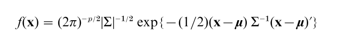
for -∞ < x_i < ∞, i = 1,…, p, where µ = ( µ₁…, µ_p) is the p-dimensional population mean vector ( -∞ < µ_i < ∞, i = 1,…, p) and Σ is the p × p population (positive definite) variance–covariance matrix. When Σ is singular, the probability density function f (x) does not exist as noted, but there are other meaningful ways to define the multivariate normal distribution.

The contours of constancy of f (x) are ellipsoids centered at µ with axes determined by the eigenvectors of Σ. Any subset of X₁,… X_p itself has a multivariate normal distribution and any set of linear combinations has a multivariate normal distribution. Also the conditional probability distribution of any subset given another subset has a multivariate normal distribution.

2.1.2 Sample Statistics And Their Properties. Suppose that a random sample X₁,…, X_N, of size N, is observed from a multivariate normal distribution. The natural estimators of µ and Σ are, respectively, the sample mean vector X and the sample variance– covariance matrix S = ∑^N_i=1(X_i – X)´(X_i – X)/(N – 1).

These estimators possess many of the properties of the univariate sample mean and variance. They are independent and unbiased; furthermore, X and [( N – 1)/N]S are maximum likelihood estimators. The sampling distribution of X is N( µ, Σ/N), and the sampling distribution of (N-1)S is called the Wishart distribution with parameter Σ and N 1 degrees of freedom, as obtained by John Wishart in 1928.

For the univariate normal distribution, when the variance σ² is known, the mean x is an optimal estimator of the population mean µ in any reasonable sense. It was shown in 1956 by Charles Stein that when p > 2, and the underlying multivariate distribution is N( µ, I), one can improve upon X as an estimator of µ in terms of its expected precision, because surprisingly, even with the identity matrix I being the population variance–covariance matrix, there is information in S to improve estimation of µ.

Authoritative references to the multivariate normal distribution and its properties include Anderson (1984) and Tong (1990).

2.1.3 Characteristic Roots. When the sample covariance matrix S has a Wishart distribution, many invariant tests are functions of the characteristic roots of S. This led to the study of the joint distribution of the roots, which was obtained simultaneously by several authors in 1939. Characteristic roots of a sample covariance matrix also play a role in physics and other fields.

The basic distribution theory for the case of a general diagonal population covariance matrix was developed by Alan James in 1956 and requires expansions in terms of zonal polynomials. For details of the noncentral distribution of the characteristic roots and zonal polynomials see Mathai et al. (1995).

2.2 Inference

Inference concerning µ when Σ is known is based, in part, upon the Mahalanobis distance N(X – µ) ∑^-1 (X – µ)´ which has a χ²_N distribution when X₁,… X_N is a random sample from N( µ, Σ). When Σ is not known, inference about µ utilizes the Mahalanobis distance with Σ replaced by its estimator vs. The distribution of the quantity N(X – µ)S⁻¹ (X – µ)´ was derived by Harold Hotelling in 1931 and is called Hotelling’s T². He showed that (N – p)T²/(N – 1)p has a standard F-distribution, F_p,N−p.

To test, at level α, the null hypothesis H₀: µ = µ₀ against the alternative H_A: µ = µ₀ based upon multivariate normal data with unknown Σ, one rejects H₀ if N(X – µ₀) S⁻¹(X – µ₀)´ exceeds (N – 1)p/(N- p)F^α_p,N−p, where F^α_p,N−p denotes the upper α-critical value of F_p,N−p. Elliptical confidence intervals for µ can be constructed as {µ: N(X – µ)S⁻¹ (X – µ) ≤ ((N – 1)p/(N – p)) × F ^α_p,N−p}. Useful rectangular confidence intervals for µ are more difficult to obtain and typically rely on suitable probability inequalities (see Hochberg and Tamhane 1987). For the univariate normal distribution, one-sided hypothesis testing straightforwardly follows from two-sided testing. However, various one-sided tests for the multivariate case are much more complicated. A particular class of techniques that is useful in this case are those of order- restricted inference.

The comparison of two multivariate normal population means, with common but unknown variance– covariance matrix, can be based upon a two-sample version of Hotelling’s T² statistic.

2.3 Linear Models: Multivariate Analysis Of Variance (MANOVA)

To compare k ( > 2) multivariate normal population means (with common unknown variance–covariance matrix), one needs to utilize generalizations of Hotelling’s T² statistic, similar to the relationship of the F-statistic for multiple populations to the two-sample t-statistic for univariate data.

To understand more generally multivariate analysis of variance, consider for the univariate setting the analysis-of-variance (ANOVA) for a given hypothesis.

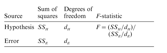
The null hypothesis reference distribution for the F statistic is F_dH,dE and the alternative distribution is a non central F-distribution; these result from SS_H and SS_E being independent random variables with SS_E ~ σ²χ²_dE and under H₀, SS_H ~ σ²χ²_dH. For example, in a one-way layout, SS­ is the sum-of-squares for treatment, and SS_E is the usual sum-of-squares for error.

The general structure of an ANOVA table for multivariate data of dimension p is parallel in structure; S_H becomes H, a p × p matrix of sum-of-squares and cross-products, and SS_E becomes E,a p × p matrix related to the variance–covariance matrix of the multivariate error vector. The random matrices H and E are independent; E has a p-dimensional Wishart distribution with d_E degrees of freedom, and under H₀, H has a p-dimensional Wishart distribution with degrees of freedom d_H.

However, now the ratio of sums of squares is translated to the eigenvalues of HE⁻¹ Because there is no uniformly best function of these eigenvalues, various alternative functions of the product, sum, or maximum of the eigenvalues have been proposed. The best-known statistics are the Wilks lambda, Hotelling- Lawley trace, Pillai trace, and Roy maximum, and are provided in standard MANOVA statistical packages.

A classical archeological example from 1935 consists of four series of Egyptian skulls ranging from the predynastic, sixth to twelfth dynasties, twelfth and thirteenth dynasties, and Ptolemaic dynasties. For each of the multiple skulls in the four series, there were measurements on breadth, length, and height. A MANOVA showed that the dynasties were not homogeneous. Subsequent analyses were carried out using multiple comparisons. The MANOVA of only two dynasty com parisons reduces to the two-sample Hotelling’s T².

3. Relationships

3.1 Regression

Regression analysis is designed to predict a measure Y based on concomitant variables X = (X₁,…, X_p). It was historically traditional to assume that (Y, X ) have a joint normal distribution with zero means and ( p + 1) × ( p + 1) covariance matrix of (Y, X ): Var(Y ) = σ₀₀, Covar(Y, X ) = Σ₁₂, Var(X ) = Σ₂₂. Then the conditional mean of Y given X = x is Σ₁₂Σ⁻¹₂₂ x´, which is a linear function of the form β₁x₁ + … +β_px_p; the conditional variance is σ₀₀ –Σ₁₂Σ⁻¹₂₂ Σ₁₂, which is independent of x, a fact that is critical in the analysis.

Although the above description involves the multivariate normal distribution, the subject of regression is usually treated more simply as ordinary linear regression involving least squares.

The more general regression model consists of a p × n matrix Y in which the n columns are independently distributed, each having an unknown p × p covariance matrix Σ, and the expected value of Y is a function of unknown parameters, namely, EY = X₁BX₂, where X₁ and X₂ are p × q and r × n matrices, respectively, and B is a q r matrix of unknown parameters which is to be estimated. This model comprises what is called the multivariate general linear model (see Anderson 1984 for details).

3.2 Correlation Hierarchy: Partial, Multiple, Canonical Correlations

If (X₁,…, X_p) is a p-dimensional random vector with covariances σ_ij, the population correlation coefficient between X_i and X_j is defined as ρ_ij = σ_ij / √σ_iiσ_jj, with the sample analogue correspondingly defined. The term co-relation was used by Sir Francis Galton in 1888. Karl Pearson introduced the sample correlation coefficient in 1896; alternative names are product moment correlation or Pearson’s correlation coefficient. Because – 1 ≤ ρ_ij ≤ 1 and ρ_ij = ± 1 only when X_i and X_j are perfectly linearly related, the correlation has become a common measure of linear dependence.

For normally distributed data, the distribution of the sample correlation was obtained in 1 915 by R. A. Fisher. The test statistic √N-2r/√1-r² can be used to test that the population correlation is zero; under this hypothesis, this statistic has a Student’s t distribution with N – 2 degrees of freedom. Fisher later obtained a transformation to z = tan h⁻¹ r), which he showed to have an approximate normal distribution with mean tan h⁻¹ ρ) and variance (N – 3)⁻¹ Consequently, the z transformation provides confidence intervals for ρ. The definitive analysis of the distribution of r and z is given by Hotelling (1953).

The population multiple correlation coefficient arises when X₂,…, X_p are used to predict X₁, and is defined as the population correlation between X₁ and the best linear predictor of X₁ based on X₂,…, X_p. A similar definition holds for the sample multiple correlation. The population partial correlation is the correlation between a pair of variables, say, X₁ and X₂, conditional on the remainder being fixed, that is, X₃,…, X_p being fixed, with a similar definition holding for the sample. See Anderson (1984) for results concerning the distributions of the sample multiple correlation coefficient and the sample partial correlation coefficient, as well as related techniques for statistical inference, in the case of normally distributed data. Canonical correlations are used to measure the strength of the relationship between two sets of variables and are described more fully in Sect. 6.2.

3.3 Measures Of Dependence

Although Pearson’s correlation coefficient is a natural way to measure dependence between random variables X and Y having a bivariate normal distribution, it can be less than meaningful for non-normal bivariate distributions. Popular and useful population measures for continuous random variables include Kendall’s τ( = 4∫^∞_-∞ F (x, y)f (x, y)dxdy -1) and Spearman’s ρ ( = 12 ∫^∞_-∞∫^∞_-∞(F (x, y) – F_X(x)F_Y (y)) f_N(x) f_Y(y)dxdy), where F (x, y), F_X(x), F_Y(y) are, respectively, the bivariate distribution function of X and Y, and the two marginal distribution functions of X, Y; and where f (x, y), f_X(x), and f_Y(y) are their corresponding density functions. Kendall’s τ can be written as 4 E(F (X, Y )) 1, where the expectation is with respect to the joint distribution of X, Y and Spearman’s rho can be written as 12 E[F (X, Y ) – F_X(X )F_Y(Y )], where the expectation is with respect to independent X and Y, with distributions F_X(x) and F_Y(y). The sample estimates of Kendall’s τ and Spearman’s rho are given in Agresti (1984). Other more theoretical approaches to measuring dependence are based upon maximizing the correlation, ρ(a(X ), b(Y)), over certain classes of functions a(x) and b(y). A classical reference is Goodman and Kruskal (1979); see also Multivariate Analysis: Discrete Variables (Overview).

A related notion is the canonical decomposition of a bivariate distribution into weighted sums of independent-like components (see Lancaster 1969).

4. Methods for Generating Multivariate Models

Many newer multivariate distributions have been developed to model data where the multivariate normal distribution does not provide an adequate model. Multivariate distributional modeling is inherently substantially more difficult in that both marginal distributions and joint dependence structure need to be taken into account. Rather straightforward univariate properties or characterizations often have many multivariate versions; however, numerous multivariate concepts have no univariate analogues. Some of the more commonly used approaches to developing models are given in the following.

4.1 Characterizing Properties

One common approach to generate multivariate distributions is to develop extensions of a specific univariate property. For instance, symmetry of the univariate distribution, that is, f (x) = f ( – x), can lead to the family of reflection symmetric or multivariate spherical distributions. Here f (x₁,…, x_p) = g(|x₁|,- …, |x_p|) or f (x₁,…, x_p) = g(x²₁ +…+x²_p) for a suitable function g. The latter family, especially when incorporating covariates, naturally leads to the class of elliptically contoured multivariate distributions (e.g., Fang and Anderson 1990).

The lack-of-memory property, which characterizes the univariate exponential distribution, has been generalized to the multivariate case, and this characterization yields the Marshall–Olkin multivariate exponential distribution. Because this distribution has both a singular and a continuous part, other purely continuous multivariate distributions with exponential marginals have been developed.

Other properties that have been used to develop multivariate distributions are independence of certain statistics, identical distribution of statistics, closure properties, limiting distributions, differential equation methods, series expansions, and conditioning methods. In some instances physical models, such as shock models, provide a method for extending univariate distributions to the multivariate case.

4.2 Mixture Methods

Mixture methods have provided successful extensions for models with non-negative random variables. The introduction of a dependence structure can be accomplished by various notions of mixing. For example, if U, V, W are independent random variables; then the ‘mixtures’ (a) X₁ = U + V, X₂ = U + W, (b) X₁ = min(U, V ), X₂ = min(U, W), (c) X₁ = U/V, X₂ = U/W generate dependent bivariate random variables. In particular, a bivariate binomial distribution, a bivariate exponential distribution, and a bivariate Pareto or F distribution can be so generated. An inherent problem with multivariate versions obtained from mixture methods, as well as other generating techniques, is that the number of parameters so introduced can be as large as p, thereby necessitating large sample sizes for estimation. For a comprehensive treatment of bivariate distributions see Hutchinson and Lai (1990).

4.3 Copulas

Another approach to providing non-normal multivariate models is based on copulas or uniform representations. We provide details for bivariate random variables; the more general case is discussed in Nelsen (1999) and Joe (1997). This approach first requires specification of the univariate marginal distribution functions F₁(x), F₂(y), and then the joint distribution is F (x, y) = U(F₁(x), F₂(y)), where U(s, t) is a two-dimensional copula. There are a number of technical conditions that the function U(s, t) must satisfy, but the basic idea is that U(s, t) is essentially the distribution function of a two-dimensional random vector whose every component marginally has a uniform distribution on [0, 1]. There are many different families of copulas; for the bivariate case, examples of copulas include the standard normal copula,

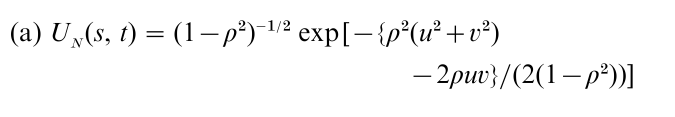
where u = Φ⁻¹(s), v = Φ^-1(t) and Φ^-1 is inverse standard normal distribution function; and the Farlie– Gumbel–Morgenstern copula,

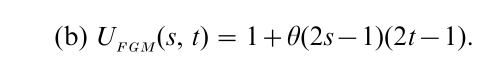
Based upon copulas like these, different multivariate distributions can be generated. For instance, the standardized bivariate normal distribution function with correlation ρ can be expressed as U_N(Φ(x), Φ(y)), whereas U_N(1 – e^−x, 1 – e^−y) has normal-like dependence structure but standard exponential distributions as its marginals. A fairly standard technique for creating copulas is to begin with any joint distribution F (x, y) and then compute F(F₁⁻¹(x), F₂⁻¹(y)), which under nonstringent technical conditions will be a copula.

Every bivariate copula U(s, t) with 0 ≤ s, t ≤ 1 satifies U⁻(s, t) = min(s, t) ≤ U(s, t) ≤ max(s + t – 1, 0) = U⁺(s, t). Both U⁻(s₁, s₂) and U⁺(s₁, s₂) themselves are copulas, and are known as, respectively, the lower and upper Frechet–Hoeffding bounds.

The probabilistic theory concerning copulas has been fairly extensively developed, but the applications to data analysis are much more limited. Copulas can be readily extended to higher dimensions. However, bounds become more complex. For more details see Ruschendorf et al. (1996).

5. Multivariate Probability Computational Techniques

5.1 Multivariate Bounds For Probabilities

Inequalities or bounds for multivariate probabilities are important tools in simultaneous inference and for approximating probabilities. We consider three basic types of inequalities, noting that for each there are numerous generalizations and extensions.

Perhaps the oldest method is based on Boole inequalities which provide relations between probabilities of events. The Frechet–Hoeffding bounds can be viewed as extensions of Boole’s inequality. In a statistical context, the lower bound of the Boole inequalities are called Bonferroni inequalities, and are often used when dealing with multiple comparisons. These bounds have many extensions; see Hochberg and Tamhane (1987), Galambos and Simonelli (1996), and Hypothesis Tests, Multiplicity of.

A second set of inequalities are called Chebyshev inequalities. For bivariate random variables X₁, X₂ with EX_i = µ_i, Var(X_i) = σ_i and correlation

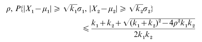
thereby extending the classical Bienayme–Chebyshev univarite inequality.

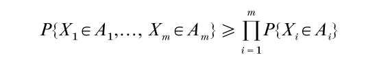
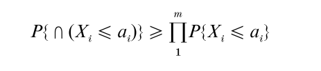
Another class of inequalities are multiplicative inequalities that hold for certain classes of random variables, namely,

When X₁,…, X_m are independent normal variates wit h respective means µ₁,…, µ_m, and common variance σ², then

where s² is an independent estimate of σ². This inequality yields a bound for the joint probability of a simple multivariate t-distribution in terms of probabilities of univariate t-distributions.

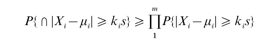
When X₁,…, X_m are correlated normal variates with a correlation matrix R = (ρ_ij) with ρ_ij ≥ 0, then the one-sided orthant is bounded

The two-sided version of the preceding holds for X_i without any non-negativity restrictions on the correlations.

For discussions of multivariate inequalities see Dharmadhikari and Joag-dev (1988) and Tong (1980).

5.2 Approximations Of Probabilities

There are a number of different numerical and stochastic techniques that are in use to obtain numerical approximations to multivariate probability statements. These techniques are useful in a variety of circumstances, for example, computing p-values for complicated multivariate data, obtaining power curves for multivariate tests, and computing multivariate posterior distributions.

Basic techniques for multivariate probability approximations rely on standard numerical integration principles; here P {xϵA} = ∫…∫_xϵA f (x)dx is approximated by ∑_{xi}w_i f (x_i), where w_i are weights and {x_i}is a finite set of points specified in A. Elementary Monte Carlo integration techniques involve random sampling N points x_i, i = 1,…, N according to f (x) and estimating P{A} by N⁻¹ ∑^N_i=1 I(x_i ϵ A), where I(x_i ϵ A) = 1, if x_i = A, and = 0, otherwise. Some methods for computing multivariate nor- mal probabilities first transform the random variables, and rewrite P{A} = ∫…∫_||z||=1 F (z)dz, where F (z) is a function defined by Σ and the region A. Then P{A} is estimated by N⁻¹ ∑^N_i=1 F (z_i) where the z_i are randomly chosen from the surface of a sphere in p-dimensional space.

Monte Carlo importance sampling techniques assume a convenient density g(•) whose support includes the support of the density f (•), and g(•) is chosen to expedite convergence. Then points y₁,…, y_N are random samples according to g(y) and P{A} is estimated by N ∑^N_i=1 I(y_i ϵ A)[ f (y_i)/g(y_i)].

More recently, Markov chain Monte Carlo methods have been developed and have proven to be particularly useful for high dimensional random vectors. The common aspects of these types of techniques is the definition of a Markov chain x₁, x₂,… which converges to a stationary Markov chain where x_i has marginal distribution f (x). Again, P{A} is approximated by (N – m + 1)⁻¹ ∑^N _{i =m} I(x_i ϵ A), where x_m,…, x_N is a suitably chosen sequence of elements generated by the Markov chain. For much more complete details, see Monte Carlo Methods and Bayesian Computation: Importance Sampling; Marko Chain Monte Carlo Methods; Monte Carlo Methods and Bayesian Computation: Overview.

6. Structures And Patterns

6.1 Principal Components

A correlation matrix represents the interdependencies among p measures, which may be likened to a connected network. The removal of one of two closely connected variables (that is, highly correlated) takes no account of how these variables are connected to the remaining measures. Principal components introduced by Harold Hotelling in 1933 (see Hotelling, Harold (1895–1973), methodology that transforms the original correlated standardized variables z₁,…, z_p into new variables z*₁,…, z*_p (called principal components), which are uncorrelated. These new variables are linear combinations of the original variables. The variance of the standardized z_i is 1, and denote the variance of z*_i by τ²_i; then the total variance p = Στ²_i remains fixed for the two systems of variables. By ordering the variances τ₍₁₎² ≥ τ₍₂₎² ≥…≥τ²_(p), and examining the cumulative proportions τ₍₁₎² /p, (τ₍₁₎² + τ₍₂₎²)/p,…, (τ²₍₁₎ +…+ τ²_(p))/p = 1, we obtain what is often called the ‘proportion of variance explained by the principal components.’ In this way we may obtain a subset of principal components that explain most of the variance, thereby providing a parsimonious explanation of the data. In effect, principal components provides a method of data reduction. The challenge in using this approach is deciding how many principal components are reasonably required and how to interpret each component.

6.2 Canonical Variables

As noted, principal components provides a procedure for the reduction of a large number of variables into a smaller number of new variables. When the variables fall into two natural subsets, as for example production and sales variables, or multiple measurements on two siblings, then canonical analysis provides another exploratory data reduction procedure. If the two sets are labeled X₁,…, X_p and Y₁,…, Y_q ( p ≤ q), canonical analysis attempts to simplify the correlational structure consisting of ( p + q) ( p + q – 1)/2 correlations to a simpler correlational structure of only p correlations.

This reduction is accomplished by forming linear combinations (U_i, V_i), i = 1,…, p, of the X_i’s and Y_j’s, respectively, with the property that all the variances are 1, ρ(U_i, V_i) = ρ_i and all other correlations are zero. The new variables are called canonical variables, and the correlations ρ_i are called the population canonical correlations.

This procedure is equally applicable to sample data. Often the first few sample canonical correlations are large compared to the remaining ones, in which case the first few canonical variables provides a data reduction procedure, which captures much of the structure between the two sets of variables.

6.3 Latent Structure And Causal Models

Latent structure models refers to a set of models that attempts to capture an understanding of causality, and hence are sometimes referred to as causal models. The term is not well-defined and at its broadest includes factor analysis, path analysis, structural equation models, correspondence analysis, loglinear models, and multivariate graphical analysis. One feature of some of these models is the description of a set of observables in terms of some underlying unobservable random quantities. Depending on the context, these unobservable variables have been called latent variables, factors, or manifest variables. See also Factor Analysis and Latent Structure: Overview.

Graphical models often provide a visual under- standing of relationships. Their origin arose in a number of scientific areas: as path analysis from genetic considerations, as interactions of groups of particles in physics, as interactions in multiway contingency tables. They are particularly useful in multivariate models because variables are related in a variety of different ways, as, for example, conditionally, longitudinally, or directly. Graphical models can be used in conjunction with specific models, for example, factor analysis, and structural equation models. For details concerning graphical models see Lauritzen (1996) and Graphical Models: Overview.

6.3.1 Factor Analysis. Factor analysis is one of the oldest structural models, having been developed by Spearman in 1904. He tried to explain the relations (correlations) among a group of test scores, and suggested that these scores could be generated by a model with a single common factor, which he called ‘intelligence,’ plus a unique factor for each test.

Factor analysis has been used in two data analytic contexts: in a confirmatory manner designed to confirm or negate the hypothesized structure, or to try to discover a structure, in which case the analysis is called exploratory. See also Latent Structure and Casual Variables; Factor Analysis and Latent Structure, Confirmatory; Factor Analysis and Latent Structure: IRT and Rasch Models; Factor Analysis and Latent Structure: Overview.

6.3.2 Path Analysis. The origins of path analysis is attributed to Sewall Wright, who from 1918 to 1934 developed a method for studying the direct and indirect effects of variables. Herein, some of the variables are often taken as causes, whereas others are taken as effects. However, because the linear relations exhibit only correlations, the view of causality remains hypothetical.

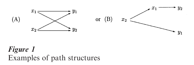
Path diagrams are typical graphical devices to show the direct and indirect variables. For example, in a study on the relation between performance and satisfaction, let x₁ be achievement motivation, x₂ be verbal intelligence, y₁ be performance, and y₂ be job satisfaction. There are several path diagrams that could exhibit these connections.

In Fig. 1A, variation in x₁ and x₂ affect both outcomes y₁ and y₂, whereas in Fig. 1B, verbal intelligence affects performance directly, and affects job satisfaction through achievement motivation.

6.3.3 Linear Structural Equations (LISREL). Structural equation models, or econometric models, were developed early on to provide explanations of economic measures. Variables whose variability is generated outside the model are called exogenous and variables explained by exogenous variables or other variables in the model are called endogenous.

A standard basic model is, for vectors x = (x₁ ,…, x_q) and y = (y₁,…, y_p) of observable variables, y = ηΛ₁ + ε, x = ξΛ₂ + δ, connected by η∆ = ξΓ + ζ where Λ₁, Λ₂ are, respectively, m × p and q × n matrices of regression coefficients; η and ξ are vectors of unobservable dependent variables, ∆ is an m m regression matrix of the effects of endogenous on endogenous variables, Γ is an m × n regression matrix of the effects of exogenous on endogenous variables, and ε, δ, and ε are residual vectors. For more details see Latent Structure and Casual Variables.

6.4 Clustering

Often, subsets of individuals are grouped by a known characteristic, as for example, by sex, by race, by socioeconomic status. In other instances, prespecified grouping characteristics may not be available. This is analogous to thinking of a galaxy of stars to be separated into groups. The methodology of clustering may be thought of as a data reduction procedure, where the reduction is to group individuals. This is in contrast to principal components or canonical analysis, in which the reduction is based upon combining variables. Alternatively, we may think of clustering as creating a classification or typology of individuals or items. For example, we may think of creating regions based on a set of demographic variables, or a set of products based on how they are used.

Suppose that the data consists of p measurements taken on each of n individual (objects). For each pair of individuals, we form a ‘distance’ measure, where ‘distance’ is flexibly defined. Thus we create an n × n matrix of ‘distances’ for which there are a variety of algorithms that govern the creation of subgroups, in part because there is no universal definition of a cluster, nor a model that defines a cluster. Intuitively, we think of a cluster as being defined by points that are relatively ‘closer’ to one another within the cluster, and ‘further’ from points in another cluster. See Statistical Clustering for more details.

6.5 Classification And Discrimination

Classification or discriminant analysis is another classically important problem in which multivariate data is traditionally reduced in complexity. Suppose that there are k populations of individuals, where for each individual we observe p variables (X₁,…, X_p). Based upon historical or ‘training’ data where we observe a sample of n_i individuals from population i, I = 1,…, k, we want to develop a method to classify future individuals into one of the k populations based upon observing the p variables for that new individual. Although fairly general procedures have been developed, it has been traditional to assume that for population i, X ~ N( µ_i, Σ), i = 1,…, k. Then µ₁,…, µ_k, Σ are estimated from the historical or training data. For a new individual, with data Z we want to optimally classify that individual into exactly one of the k populations.

The case k = 2 yields a linear classifier involving Z called Fisher’s linear discriminant function, and the case k > 2 involves k linear functions of Z.

To handle settings where we do not assume under- lying normal populations, there is the technique of logistic discriminant analysis, which again results in a linear discriminant function for two populations. More recent techniques allow nonlinear discriminant functions and nonparametric discriminant functions having a monotonicity property. The classification and regression-tree (CART) approach yields a branching decision tree for classification; see Breiman et al. (1984). Decision tree analyses have found many uses in applications, e.g., for medical diagnostics. For further information on discrimination see Multivariate Analysis: Classification and Discrimination.

6.6 Multidimensional Scaling

From a geographical map, one can determine the distances between every city and every other city. The technique, called multidimensional scaling (MDS), is concerned with the inverse problem: Given a matrix of distances, how can we draw a map? The distances are usually in p-dimensional space, and the map is in q < p dimensional space, so that MDS can be thought of as a dimension reduction technique. Further, q = 2 is the most natural dimension for a map. However, we know from the many projection procedures for drawing a map of the globe ( p = 3) in q = 2 dimensions that the resulting maps differ in how one perceives distances. For more details see Scaling: Multidimensional.

6.7 Data Mining

Data mining refers to a set of approaches and techniques that permit ‘nuggets’ of valuable information to be extracted from vast and loosely structured multiple data bases. For example, a consumer products manufacturer might use data mining to better understand the relationship of a specific product’s sales to promotional strategies, selling store’s characteristics, and regional demographics. Techniques from a variety of different disciplines are used in data mining. For instance, computer science and information science provide methods for handling the problems inherent in focusing and merging the requisite data from multiple and differently structured data bases. Engineering and economics can provide methods for pattern recognition and predictive modeling. Multivariate statistical techniques, in particular, clearly play a major role in data mining.

Multivariate notions developed to study relationships provide approaches to identify variables or sets of variables that are possibly connected. Regression techniques are useful for prediction. Classification and discrimination methods provide a tool to identify functions of the data that discriminate among categorizations of an individual that might be of interest. Another very useful technique for data mining is cluster analysis that groups experimental units which respond similarly. Structural methods such as principal components, factor analysis, and path analysis are methodologies that can allow simplification of the data structure into fewer important variables. Multivariate graphical methods can be employed to both explore databases and then as a means for presentation of the data mining results.

A reference to broad issues in data mining is given by Fayyad et al. (1996). Also see Exploratory Data Analysis: Multivariate Approaches (Nonparametric Regression).

7. Further Readings

This research paper and related entries provide only a brief overview of a vast field. For further general readings see Anderson (1984), Dillon and Goldstein (1989), Johnson and Wichern (1999), Morrison (1990), Muirhead (1982); for detailed developments see the Journal of Multivariate Analysis.

Bibliography:

1. Agresti A 1984 Analysis of Ordinal Categorical Data. Wiley, New York
2. Anderson T W 1984 An Introduction to Multivariate Statistical Analysis, 2nd edn. Wiley, New York
3. Breiman L, Friedman J H, Olshen R A, Stone C J 1984 Classification and Regression Trees. Wadsworth, Belmont, CA
4. Dharmadhikari S W, Joag-dev K 1988 Unimodality, Convexity, and Applications. Academic Press, Boston
5. Dillon W R, Goldstein M 1989 Multivariate Analysis: Methods and Applications. Wiley, New York
6. Fang K-T, Anderson T W (eds.) 1990 Statistical Inference in Elliptically Contoured and Related Distributions. Allerton Press, New York
7. Fayyad U M, Piatetsky-Shapiro G, Smyth P, Uthurusamy R (eds.) 1996 Advances in Knowledge Discovery and Data Mining. American Association for Artificial Intelligence MIT Press, Cambridge, MA
8. Galambos J, Simonelli E 1996 Bonferroni-type Inequalities with Applications. Springer-Verlag, New York
9. Goodman L, Kruskal W 1979 Measures of Association for Cross Classifications. Springer-Verlag, New York
10. Hochberg Y, Tamhane A C 1987 Multiple Comparison Procedures. Wiley, New York
11. Hotelling H 1953 New light on the correlation coefficient and its transform. Journal of the Royal Statistical Society, Series B 15: 193–225
12. Hutchinson T P, Lai C D 1990 Continuous Bivariate Distributions, Emphasizing Applications. Rumsby Scientific Publishing, Adelaide, South Australia
13. Joe H 1997 Multivariate Models and Dependence Concepts. Chapman & Hall, London
14. Johnson R A, Wichern D W 1999 Applied Multivariate Statistical Analysis, 4th edn. Prentice-Hall, New York
15. Lancaster H O 1969 The Chi-squared Distribution. Wiley, New York
16. Lauritzen S L 1996 Graphical Models. Oxford University Press, Oxford, UK
17. Mathai A M, Provost S B, Hayakawa T 1995 Bilinear Forms and Zonal Polynomials. Springer Verlag, New York
18. Morrison D F 1990 Multivariate Statistical Methods, 3rd edn. McGraw-Hill, New York
19. Muirhead R J 1982 Aspects of Multivariate Statistical Theory. Wiley, New York
20. Nelsen R B 1999 An Introduction to Copulas. Springer, New York
21. Ruschendorf L, Schweizer B, Taylor M D (eds.) 1996 Distributions with Fixed Marginals and Related Topics. Lecture Notes – Monograph Series, Vol. 28, Institute of Mathematical Statistics, Hayward, CA
22. Tong Y L 1980 Probability Inequalities in Multivariate Distributions. Academic Press, New York
23. Tong Y L 1990 The Multivariate Normal Distribution. Springer-Verlag, New York