Labor Supply Research Paper

The questions above stress work ‘for pay.’ This excludes voluntary work and unpaid household work. In fact, data are available on both voluntary work (see Freeman 1997) and household work (see Juster and Stafford 1991), and the very same conceptual framework summarized below that is used to study paid work is also employed to understand these other types of work. However, this research paper concentrates on work for pay and, subsequently, whenever the word ‘work’ is used, it should be understood that ‘work for pay’ is meant. Most of the research by economists during recent decades has addressed the supply of labor to the labor market as a whole, not the supply of labor to particular occupations or to particular firms or industries. Research on labor supply to particular occupations or to particular firms uses models similar to the one sketched below to understand the supply of labor to the entire labor market, although there will necessarily be some differences in the analysis. For a review of some research on occupational labor supply, see Freeman (1986). For a study of the labor supply to a single firm, see Nelson (1973). In this research paper, the research reviewed concerns the supply of labor to the labor market as a whole.

1. Key Empirical Regularities

Any satisfactory theory of work behavior should explain the following empirical regularities:

(a) Men work more than women.

(b) In North America and Western Europe, white men work more than black men.

(c) In recent years and in relatively rich economies, those who have been at school longer work more.

(d ) Unmarried men work less than married men while, until recently at least, married women work less than unmarried women.

(e) Work hours and employment–population ratios fall in recessions and rise in booms though this pro-cyclical movement is stronger for low-skill than high-skill workers.

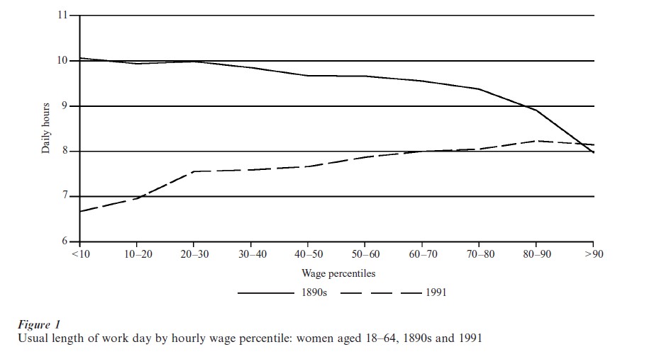
( f ) Over the past century, in North America and Western Europe, for most types of workers, work hours have fallen and vacations have lengthened. A particularly instructive illustration of this for the USA is provided in Fig. 1, which graphs the usual length of the workday by wage decile. The unbroken line in this graph draws upon information from various surveys in the 1890s while the broken line provides information from a special Current Population Survey in 1991. The length of the workday has fallen for all workers except those at the highest wage decile. Indeed, whereas low- wage workers once worked the longest hours, high- wage workers now tend to do so. Figure 1 describes US women, but the data for US men are similar (see Costa 1999a).

(g) Among men, work rises with age until middle age and then falls.

(h) Although comparisons across countries are frustrated by differences in data collection methods and definitions, it appears that, in the 1990s, average hours worked in the USA exceeded those in Europe.

(i) Average hours worked by self-employed people tend to exceed those by employees (see Aronson 1991). No doubt, instances will be found where these patterns are contradicted, but these empirical findings constitute the norm. A rich literature exists in economics on these issues.

One empirical regularity has received much less attention, the fact that individuals synchronize their work schedules: almost 80 percent of full-time workers in the USA start work between 7 a.m. and 9 a.m. and about the same proportion finish between 3 p.m. and 6 p.m. (Mellor 1986); about 60 percent of all those employed do not work weekends (Smith 1986). Presumably there are strong complementarities in work and leisure activities (i.e. the benefits to one individual from engaging in a given activity are greater if other individuals also engage in that activity at the same time) although little research effort has been directed towards identifying the key complementarities. Weiss (1996) has been one of the few to grapple with this issue.

2. An Informal Statement

2.1 Classifying The Variables

In essence, economists think in terms of an individual’s time spent at work as depending upon four classes of variables: (a) pay per unit time at work; (b) other income; (c) certain demographic characteristics that are observed by researchers; and (d) characteristics of the individual that are unobserved by researchers.

Consider these variables in turn. First, the dependent variable: time spent at work. There are many different dimensions of work time, including annual hours of work, annual weeks worked, weekly hours, daily hours, and whether to work or not.

Now the independent variables. ‘Pay per unit time at work’ is designed to measure the incentive to work or, equivalently, the price of not working. It is usually measured by an individual’s average hourly earnings. Economists usually presume that after-tax earnings matter, not pre-tax earnings. Where average hourly earnings do not vary with time at work, then the use of hourly earnings is appropriate to characterize the incentive to work for pay. However, there are a number of instances where the wage per hour is not fixed but varies (often increases) with work hours so average hourly earnings may provide only a local indicator of work incentives. For instance, in many countries, by statute or by union-negotiated collective bargaining agreements, or by the operation of market forces, wage premiums are paid for long hours worked per week. Or job offers come in tied wage-hours packages: one employer may offer a job specifying a wage of US$10 per hour for 40 hours per week while another may specify a wage of US$12 per hour for 42 hours. In these instances, the incentive to work is not provided by a single wage rate that describes all work opportunities.

The variable ‘other income’ is sometimes represented by the individual’s rent, dividends, and interest, so-called nonlabor income. This type of income for an individual is often the consequence of labor income earned at an earlier age and, therefore, will tend to be higher for those who habitually work long hours. In this way, high non-labor income will tend to be a result of, rather than a cause of, long work hours. Hence, some researchers prefer to use some measure of wealth at a young age (if the data are available to measure it). Or ‘other income’ is sometimes represented by the labor income of other family members.

It is routine to examine the relationship between time at work and wages holding constant certain demographic characteristics, such as gender and race, characteristics that are typically included in surveys and that are available to researchers. Even allowing for differences in wages and other income, work patterns vary by race and gender, suggesting either systematic differences in ‘tastes for work’ or different work and nonwork opportunities for these groups.

Finally, it is recognized that much of the variation in work behavior across individuals remains unaccounted for after holding constant all the variables that are usually provided in large data sets. Expressed differently, variables unobserved by researchers ‘explain’ most of the variation in work across individuals. These unobservables are sometimes called ‘tastes for work,’ but it should, be understood that this is simply giving a name to our ignorance.

2.2 The Nature Of The Available Data

It is important in understanding any empirical labor supply research to recognize the essential source of variation in the data that is being exploited to measure the effects of various variables on work. One source of variation is across people: the correlation between work and other variables (especially wages and other income) is computed across people observed at approximately the same time. This correlation is often calculated separately for men and women and for different racial groups. A different source of variation is over time: here, in essence, the average values of each individual’s work and other variables are first computed, then variations over time around each individual’s average in work and other variables are calculated to form the relevant correlations.

Although it is straightforward to compute these correlations, they are sometimes difficult to interpret. Consider the effect of wages on work behavior, a subject that has been the focus of most of economists’ research on labor supply. An ideal experiment from which to infer the effect of wages on work would be to select people in the population at random, assign wages to them prior to their work choices, and then observe whether and how much they work. In this experiment, the parts played by the random selection of the population and the prior assignment of wages to people are very important. Unfortunately, nature does not provide us with these ideal experimental conditions.

First, the wages that people face at any moment are determined in part by individuals’ past decisions about how long to stay at school and what skills to acquire. These past schooling and training decisions may have been made with the expectation of capitalizing on them subsequently by working longer hours in the labor market. People who are less averse to market work are more likely to stay at school longer and to acquire the skills that result in relatively high wages later in life. In this event, the correlation between work hours and wage rates incorporates a causation that runs from preferences about work hours to wages rather than the other way around. Wages are not assigned to people in the manner described by our ideal experiment; in part, wage differences across people reflect people’s prior decisions and their past and current preferences.

Second, when computing the correlation between work hours and wage rates, the wage rates facing people who choose not to work for pay are usually unobserved. Expressed differently, information on the wage offers that nonworkers are rejecting is not available to researchers. This problem is typically addressed by computing the hours–wage correlation among those working positive hours only. However, this generates the problem that the sample of people who choose to work does not represent a random sample of the population but a highly nonrandom and self-selected sample. The requirement of our ideal experiment that the correlation between work and wages be computed for people who constitute a random sample of the population is not met. This is one manifestation of what has become known as the problem of ‘sample selection’ and it has been emphasized in Heckman’s influential research (e.g. Heckman 1979). The sample selection problem arises whenever factors unobserved by the researcher affect both (a) the selection of the sample over which the hours–wage correlations are to be computed and (b) the hours of work decisions of the individuals. In this case, the ideal experimental condition—the random selection of the sample—is not being satisfied, and the meaning of the hours–wage correlation is subject to more than one interpretation (as shown succinctly by Heckman 1993).

Therefore, the data available to researchers to compute the effect of wages and other variables on work behavior probably do not satisfy certain ideal experimental conditions and this frustrates measuring the behavioral parameters governing the impact of these variables on work choices.

3. Static Models Of Labor Supply

3.1 Conceptual Framework

To model an individual’s work decision, let his or her preferences for work hours (h) and consumption (c) be embodied in a utility function U=U(c, h; X, e) where X denotes fixed characteristics of the individual such as gender and race that are observed by researchers. Characteristics affecting preferences that are not observed by researchers are given by e. The individual’s income–expenditure constraint is expressed as p·c=w·h+y, where p is the price of consumer goods, y is nonlabor income, and w is average hourly earnings.

In the simplest and most tractable of cases, p, w, and y are fixed to the individual and independent of choices of c and h. In this instance, provided U has some convenient technical properties, selecting c and h to maximize U subject to the income–expenditure constraint yields an expression that relates hours worked, h, to the budget constraint variables that are given to the individual, namely, p, w, and y, and to the fixed characteristics conditioning his preferences, X and e: h=f ( p, w, y; X, e). This relationship is the labor supply function and it provides a formal justification for the characterization given in Sect. 3, whereby time spent at work is related to four classes of variables: w, y, X, and e. (Because the budget constraint may be written c=(w/p)·h+( y/p), it is evident that there are not three independent price and income variables, namely, p, w, and y, but only two such variables, namely, w/p and y/p.) As usual in economics, for the key empirical propositions, it is not essential that any individual behaves in this easily caricatured, maximizing manner, but that it facilitates the derivation of relationships and provides a convenient benchmark if we assume that the individual behaves as if he were deliberately optimizing. Less terse explanations of this model can be found in many good textbooks such as Ehrenberg and Smith (1997) or Filer et al. (1996).

This framework applies to the individual who chooses to work a positive number of hours (h>0) and to the individual who chooses not to work at all (h=0). In the case of the decision of whether to work, the individual who is currently not working compares the wage per hour he would receive if he worked, the ‘offered market wage,’ with his reservation wage which is defined as the implicit value of his nonwork time. When his reservation wage exceeds his offered wage, he does not work for pay (h=0); when his reservation wage falls short of his offered wage, he works some positive hours in the market (h>0). Therefore, the higher is the offered wage, the greater the likelihood of an individual working for pay.

The previous statement concerns an individual’s work decisions. Many people live in households where joint work decisions have to be made. In these cases, the standard treatment postulates a household utility function that depends upon the household’s consumption and the work time of each household member. If incomes and expenditures are pooled, then each household member’s work behavior will depend not only on his wage rate but also on the wage rates of other household members.

This household formulation has been the subject of criticism in recent years for failing to specify how the household utility function is derived and for being silent on how resources are allocated within the household (see, for instance, Chiappori 1988). Recent models start with the utility functions of each household member and postulate that the household reaches efficient decisions with respect to its consumption and work behavior. ‘Efficiency’ here means that, given prices and wages, the work and consumption decisions of the household members have exploited all opportunities to enhance their welfare without cost so that one person’s welfare can be improved only by lowering another member’s welfare.

One version of these models characterizes household decision making as a bargaining process. Each individual has a level of welfare that can be enjoyed in the absence of cooperation with other members of the household. This is the individual’s ‘threat point’ and is sometimes equated with the welfare the individual would enjoy if he or she left the household. Provided the household remains intact, anything that increases an individual’s threat point will increase the individual’s share of the benefits from remaining in the household. For instance, if the market wages paid to unmarried women rise, this increases the wife’s threat point in bargaining with her husband and, provided the wife remains married, she should enjoy a greater share of resources within the household. This model has been used not only to understand husband–wife decision making and the growing incidence of divorce, but also intergenerational behavior in developing countries when adult children live with their parents. A formal treatment of these issues is found in McElroy (1990) and a more accessible discussion is in Lundberg and Pollak (1996). These models are likely to be a popular topic for future research especially if they are able to add materially to our understanding of household formation and dissolution.

3.2 Empirical Research

A large amount of empirical research has been directed towards the relationship between h and w. This is because changes in income taxes and other sorts of taxes and changes in welfare benefits are tantamount to changes in w (and sometimes in y, too) and the cost and benefits of these tax and welfare policies depend critically on whether and by how much hours worked and employment–population ratios increase or decrease as w is altered.

In labor economics research in the 1970s and 1980s, the most common source of information to examine the relationship between hours worked and average hourly earnings consisted of large cross-sectional data sets, that is, data on individual people observed at approximately the same calendar time. In essence, after controlling for differences among people in many characteristics, the residual correlation was computed between time spent at work and average hourly earnings. In other words, the impact of wages on work was inferred from differences among people in their wages and work after controlling for other variables.

The most common finding in this research was that, among adult men, hours worked and wage rates were mildly negatively correlated while, among adult women, hours worked and wage rates were positively correlated. A summary and evaluation of these studies appear in Killingsworth (1983), Pencavel (1986), and Killingsworth and Heckman (1986). However, the particular results were disturbingly fickle: relatively small changes in the composition of the sample or in estimating methods sometimes had large effects on the magnitude of the work–wage correlations. Mroz (1987) provides an excellent demonstration of this. Recent research has tended to yield somewhat more consistent and robust results. This is because the more recent research has followed people over time so, in addition to the variation in the data across people, there is also variation in the data for each person over time. When understanding such intertemporal variation, it becomes important to consider life-cycle or dynamic models of labor supply.

4. Life-Cycle Models Of Labor Supply

In life cycle models of the effect of wages on work behavior, it is crucial to ask: What is the source of the variation in observed wages to which individuals are adjusting their labor supply? One source of variation is the life-cycle variation in wages for a given individual, that is, the evolutionary changes in wages as a person ages. Typically, as an individual ages, their wages rise, sometimes at a decreasing rate, until later in life when wages begin to fall. A second source of variation in wages is the difference in wages across people at the same stage in their life cycle. This second source of variation in wages is called the parametric difference in wages across individuals. At any moment, differences in work behavior among people will be a mixture of responses of labor supply to, first, the path of wages as a given individual ages and, second, differences across individuals in wages observed at the same age.

The first of these responses may be observed if the work behavior and wages of a cohort of people born at about the same time are followed as they age. The proportional change in hours worked that follows a proportional change in wages as these individuals age is called the intertemporal substitution elasticity. It is the life-cycle effect of wages on work. Instead of following people born at about the same time, sort these individuals by age group and compute the correlation between work and wages across people within each age group. These people are about the same age, but they are born in different years (as they belong to different cohorts) so that the observations on their work and wages must be drawn from different calendar years. This correlation incorporates the response of labor supply to parametric differences in wages across people.

The first study to lay out these distinctions with clarity and to compute the various labor supply responses was MaCurdy (1981). His estimates of the intertemporal substitution elasticity for adult US men were in the order of 0.23, meaning that a 10 percent growth in wages as an individual ages would induce a 2.3 percent increase in annual hours worked. His estimates were imprecise, but more recent estimates for both men and women derive similar values for the intertemporal substitution elasticity (see Pencavel 1998, 1999).

When individuals are sorted by age and the correlation between work and wages computed across people holding age approximately constant, the subsequent estimate of the impact of wages on work is often (though not invariably) positive: for both US men and women, a representative estimated elasticity of annual hours with respect to wages is of the order of 0.10. (The elasticity of hours with respect to wages is defined as the proportional change in hours induced by a proportional increase in wages.)

Whereas in the research in the 1970s and 1980s it was common to compute negative estimates of labor supply elasticities, in the 1990s the estimates were more frequently positive and appeared less sensitive to modifications in specification and methods. Why should this be? First, there is a better understanding about the need to distinguish conceptually among different possible wage effects on work behavior. In particular, researchers differentiate the incentives for an individual to work at ages when his wages are relatively high (this is the life-cycle effect) from the incentives to work that come from wage differences arising for reasons that are independent of age (this is the effect of parametric differences in wages). Second, the 1990s research had an important time-series dimension, which may be a critical feature given that, over the past 20 years or so, the structure of wages has changed considerably. This generates a variation in wages that was denied to researchers in the 1970s and 1980s who relied exclusively on wage differences among people at a given moment.

Though there remains some disagreement among economists regarding the value of the elasticity of hours worked with respect to wages, it is undeniable that positive estimates of the effect of wages on work would help to explain many features of changes in work behavior over the past 25 years in the USA. Work levels have increased more for women than men, they have increased more for well-educated people than poorly educated people, and they have increased more for married people than for single people. In each of these three comparisons, the wage structure has changed favoring those who work more: the wages of women have risen relative to those of men, the wages of well-educated workers have risen relative to those with less education, and the wages of married people have risen relative to the wages of unmarried people. One simple story compatible with these facts is that changes in technology and other factors have caused changes in the wage structure and—if work–wage relationships are positive—these wage changes have induced relatively more work from those whose wages have risen relative to those whose wages have fallen.

Positive work–wage estimates may also explain some of the empirical regularities listed in Sect. 2. Men work more than women and, other things equal, men are paid more per hour than women. White men work more than black men and, other things equal, white men are paid more than black men. Those with more schooling work more and those with more schooling have higher average hourly earnings. Unmarried men work less than married men, and unmarried men tend to have lower wages than married men. Unmarried women work more than married women, and unmarried women tend to have higher hourly pay than married women. The work–age patterns for men broadly correspond to their wage–age patterns. No doubt, there are other competing explanations for these regularities, but the naıve positive association between work and wages across these groups is striking.

5. Other Empirical Findings

5.1 Labor Supply And Taxes

One aspect of labor supply research that has occupied a large amount of attention is the impact of income taxation on work behavior. If t is the tax rate, w represents gross (that is, pre-tax) hourly earnings, and y is gross ( pre-tax) nonlabor income, then net or posttax wages are defined as wⁿ=(1-t)·w and net or post-tax nonlabor income is yⁿ₌ (1-t)·y. If each individual responds to net wage rates and net nonlabor income, then the relevant budget constraint involves the post-tax variables: p·c= wⁿ ·h+yⁿ.

The problem posed for researchers measuring the effect of income taxes on labor supply is that, in most income tax systems, tax rates change with income (which, in turn, changes with work hours) so that the net wage rate varies as an individual alters his work hours. This means that the incentive to work is not represented by a value for hourly earnings that is fixed to the individual and independent of their work choice. Instead, there is no single value that represents the incentive to work because the net hourly wage at, say, 20 hours of work per week will diverge from the net hourly wage at 40 hours per week. In this instance, the budget constraint, p·c= wⁿ ·h+yⁿ, is no longer linear.

It is not only the explicit income tax system that produces nonlinearities in the budget constraint. Most income-maintenance programs designed to provide support for low-income people also result in nonlinear budget constraints for individuals eligible for such programs. This is because most income-maintenance programs do not transfer a fixed sum that is independent of the recipient’s income. On the contrary, most transfer programs are income conditioned: less money is transferred to the recipient as the recipient’s income rises, until a point is reached, the so-called break-even point, where transfers are reduced to zero and the individual moves off the welfare program and is faced with just the ( positive) income tax system. The rate by which transfer income is reduced as the welfare recipient earns one more dollar is the welfare system’s implicit tax rate. Virtually all implicit tax rates are very high, often as high as 100 percent when transfer income is reduced by one dollar for every dollar that the individual earns, so that budget constraints of lowincome people are highly nonlinear.

The research on the labor supply effects of income taxes and transfers tries to reproduce the essential features of individuals’ after-tax and after-transfer budget constraints. When the tax system can be characterized as generating an after-tax budget constraint for an individual in which after-tax wage rates are continually falling as more hours are worked (that is, a budget constraint that is strictly concave from below as implied by a smoothly progressive tax system), the statistical procedures for estimating the effect of wages and taxes on work behavior are relatively straightforward and tractable. When, however, the after-tax budget constraint has kinks and net wages may rise over some regions as hours increase, the statistical methods become more recondite and the results more sensitive to alternative estimation methods. The variation in the estimates of different studies reported in Blundell and MaCurdy’s (1999) survey is striking. The essential source of the difficulty for researchers is that most data sets provide little information about the income tax and transfer pro- grams that households face. Consequently, with the information available on gross wages and income, in effect, researchers try to complete the income tax and transfer algorithms for each individual, but the in- accuracies in this process and the errors introduced must be extensive.

A similar problem exists in trying to determine the impact of welfare or income maintenance programs on labor supply. A popular hypothesis is that some people reduce their work levels and, therefore, their market earnings to become eligible for welfare. This is revealed, it is argued, by the fact that welfare participation (the fraction of households receiving welfare payments) is higher in those states in the USA where the welfare program parameters imply relatively generous benefits. The problem with this argument is that, even in the absence of any work incentive effects of the welfare system, an association between welfare participation and the parameters of the welfare system are to be expected. Where welfare program parameters imply relatively generous welfare benefits, households will accept opportunities to raise their disposable income and participate in the welfare program, even if they do not change their work behavior. The association between welfare participation and welfare program parameters (especially the welfare system’s implicit tax rate) has to be specified carefully to identify work incentive effects (see Ashenfelter 1983). Unfortunately, because very few differences across states exist in the statutory implicit tax rate on welfare income, there is little persuasive evidence from welfare programs of work disincentive effects.

Therefore, at present, probably the most reliable estimates of the effect of income taxes and transfers on work behavior are those inferred from studies that compute the impact of changes in gross wages on work. The assumption here is that the effect of a proportional increase in gross wages on work hours equals the negative of the effect of a proportional increase in tax rates on work hours. This implies, given the estimates reported above of the impact of wages on work, that a 10 percent increase in income tax rates will induce individuals belonging to one cohort to work between one and three percent fewer hours at each age than they would otherwise choose to do.

5.2 Family Labor Supply Decisions

The employment probabilities of husbands and wives do not appear to be independent of one another. To show this, consider caucasian households in the USA where both the husband and the wife are aged between 25 and 64 years. (The data are drawn from the 1960 Census of Population.) Table 1 presents the joint and unconditional probabilities of market work of these husbands and wives. Thus, the probability that both the wife and the husband work is 0.557 and the probability that the wife works but the husband does not is 0.059. Hence the sum of these two joint probabilities is the unconditional probability of the wife working which is 0.616 (given in the bottom line of Table 1). Similarly the probability that the wife does not work but the husband does is 0.309 and (as already noted) the probability that both the wife and the husband work is 0.557. Hence, the sum of these two joint probabilities yields the unconditional probability of the husband working which is 0.866 (given in the last column of Table 1).

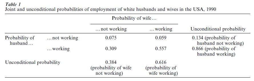
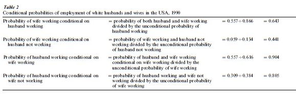
From these joint and unconditional probabilities can be derived the conditional probabilities and these are listed in Table 2. For instance, the probability that the wife works conditional on the husband working is 0.643, given in the first line of Table 2. Or, the probability that the husband works conditional on the wife also working is 0.904 given in the third line of Table 2. If the husband’s and wife’s employment probabilities were independent, then the conditional employment probabilities in Table 2 would equal the unconditional probabilities in the final column and the final line of Table 1. In fact, the conditional probabilities of the wife working are 0.643 and 0.441 (given in the first two lines of Table 2) whereas the unconditional probability of the wife working is 0.616 (from Table 1). The conditional probabilities of the husband working are 0.904 and 0.805 (given in the last two lines of Table 2) while the unconditional probability of the husband working is 0.866 (from Table 1). These data suggest that employment independence is closer to being satisfied for husbands than it is for wives. However, for both husbands and wives, the probability that one is employed is greater if his or her spouse is also employed. Consistent with this, working husbands and wives tend to retire at or close to the same time (see Hurd 1990 and Costa 1999b).

There are a number of reasons why employment probabilities of husbands and wives are positively correlated. First, this may reflect something about marital choices: women less averse to market work tend to marry men with similar work preferences. Second, the correlation may be that each party’s responses to their shared economic environment. For instance, if both husbands and wives work more in households possessing little nonlabor income, then the positive correlation in work behavior may reflect the common influence of this source of wealth. Third, the correlation may be the outcome of both marriage patterns and economic environments. For example, it has already been reported that those men facing higher wages are more likely to work in the market than lower wage men and those women facing higher wages are more likely to work in the market than lower-wage women (a). Furthermore, high-wage men tend to marry high-wage women (b). Together, (a) and (b) will generate a positive correlation between the employment probabilities of husbands and wives.

The positive correlation in the market work of husbands and wives may also reflect cross-wage effects. That is, hold the wages of the husband constant: then, do those husbands married to relatively high-wage wives work more than those husbands married to relatively low-wage wives? Conversely, hold the wages of the wife constant: do those wives married to relatively high-wage husbands work more than those wives married to relatively low-wage wives? This issue has arisen in the last few decades as a possible reason for the growth in the employment–population ratio of married women. A popular explanation has focused on the slow growth in the wages of married men since the early 1970s: are married women working more because the wages of their husbands have increased so little or, in some instances, have actually decreased? The broad trends in the key variables support such an interpretation because there has been a steady increase in the market work of married women while, for the past 25 years or so, median real wages of married men have increased hardly at all.

Indeed, the work decisions of husbands and wives do seem to be related to the wages of their spouses. In particular, when one spouse’s real pay falls, the other spouse tends to work more (see Juhn and Murphy 1997, Pencavel (1998, 1999)). However, these cross-wage effects—the relation between one individual’s work behavior and his or her spouse’s real earnings– are much less powerful than the own-wage effects (that is, the relation between each individual’s work behavior and his or her own real wages). According to these findings, the employment of married women has increased principally because their real offered wages have been increasing and the movements of their husband’s earnings have been a factor, but a factor of less importance in accounting for the movements in their work levels.

If women were working more to augment the stagnant pay of their husbands, then the increases in the work of married women should be greatest for those men whose wages have fallen, not for those men whose wages have risen. In fact, the largest increases in work among women have occurred for those women married to high-wage men and the real earnings of high-wage men have tended to increase in real terms since the 1970s. By contrast, the market work of wives of low-wage men has increased much less and yet the real wages of low-wage men have tended to fall. These facts are reported in Juhn and Murphy (1997).

Hence this evidence suggests that husbands and wives tend to substitute their work time for one another: when the wage rate of one party increases (decreases), that person works more (less) and his wife or her husband works less (more). The positive correlation in the employment probabilities of husbands and wives is driven more by marriage patterns and by own-wage effects than by cross-wage effects.

5.3 Work Behavior Of Older People

One of the most striking of long-term developments in work behavior is the decline in employment of older men. Of men 65 years and older, 68 percent were in the labor force in 1890, 42 percent in 1940, 31 percent in 1960, and fewer than 20 percent in the mid-1980s. Interestingly, from the mid-1980s to the mid-1990s, this decline appears to have flattened out. Similar declines in hours of work among those men employed are also observed. By contrast, the labor force participation rate of women aged 65 years and over has changed very little: it was 8 percent in 1890 and a little more than 8 percent 100 years later.

The drop in the amount of work allocated by older men to the market is one definition of retirement. Another definition, often accompanying the first, turns on the receipt of pension or Social Security income. It is tempting to convert this association into a causal relationship: retirement in the sense of the reduction in labor supply among older workers is induced by the opportunity to draw on annuities from accumulated pension funds.

Because the dominant retirement income for the median elderly household is Social Security income, a much researched issue has been the impact of Social Security on retirement. For most of the past 50 years or so, Social Security wealth has been increasing over time while male labor force participation rates have been falling so the aggregate time-series movements in these variables are compatible with a causal role for public pensions. However, monthly income from Social Security was first paid in 1940 to a relatively small fraction of the elderly population at which time labor force participation rates of men 65 years and over had already fallen by more than 20 percent since the beginning of the century. As Costa has noted (1998, pp. 20–21), in the USA and other countries (Britain, Germany, and France), retirement trends do not display a discontinuity around years when, as a consequence of new legislation, public pension benefits start being paid.

However, a role for Social Security affecting retirement behavior is suggested from an examination of the retirement patterns of the members of a given cohort as they age. In particular, since the mid-1960s when early Social Security benefits were first introduced, there has been a spike in male labor force participation rates at age 62 years. It is difficult to understand why there should be such a spike at 62 years other than the discontinuous retirement incentives embodied in the Social Security benefit rules.

In addition, certain private pension programs create incentives to retire before the age of 65 years. Thus, defined-benefit pension plans specify the pension annuity as a fixed proportion of a worker’s highest annual earnings and often the actuarial value of such defined-benefit plans is higher for people younger than 65. The fraction of workers covered by defined-benefit pension programs has been falling and that of defined- contribution pension plans increasing. Because pension wealth grows until the funds are withdrawn, defined-contribution plans embody no incentives for early retirement.

The growth in Social Security and in private pensions represent specific manifestations of a more general phenomenon, namely, the increase in wealth that many cohorts have enjoyed this century. This increase in wealth discourages market work at some time during an individual’s life and it may be efficient for the typical individual to take this increased leisure not in the form of fewer work hours each year, but in the form of fewer years at work and of earlier retirement.

5.4 Differences In Work–Wage Elasticities

In undergraduate textbooks, for many years it has been common to draw graphs of the relationship between hours worked and wages that imply a positive association at relatively low wages and a negative association at relatively high wages. This nonlinear relationship is called a ‘backward bending labor supply curve.’ Although this curve is a staple of every economics student’s education, the empirical support for this relationship is meager. In some instances, researchers have specified the relationships in such a way that a nonlinear and nonmonotonic relationship between wages and work hours was not investigated. In other instances, however, researchers have explored the possibility of this backward-bending curve and found little evidence for it.

With the richer, more recent, data that combine cross-section and time-series variation, the issue has come up for re-examination. It surfaced because the impact of wages on work appeared to be larger for men with relatively low levels of schooling than for well-educated men, and it was a short step to move from this observation to a specification in which the impact of wages on labor supply fell as wages rose. Indeed, according to one set of estimates, the elasticity of annual hours worked with respect to wages is calculated to be of the order of 0.33 at the average wage of men with less than a high school education, and it falls to 0.14 at the average wage of men with more than 16 years of schooling (see Pencavel 1999). Note, however, that although the slope of the hours– wage relationship becomes less positive at higher wages, it never becomes negative, except for a very few people with extremely high wages. A similar result is obtained by Juhn and Murphy (1997).

6. Conclusion

Over the past 40 years or so, there has been a very large volume of research on labor supply by economists. This is because the work decisions of individuals represent one of the essential components of labor market analysis (in the classical metaphor, these labor supply decisions represent ‘one blade of the scissors,’ the other blade being the hiring and employment decisions of firms) and because questions involving labor supply are closely tied to important issues of the public policy (such as the effect of income taxes on how much individuals work). This research has been increasingly sophisticated in economic and statistical modeling. In addition, much more is known today about work patterns than was known in 1960. Some components of the economist’s standard model of labor supply (such as the intertemporal substitution elasticity) have been estimated with confidence. However, there remains some disagreement over the values of other key parameters such as the effect across different individuals of increases in wages on hours worked. Most economists probably believe that, for the typical worker, increases in wages generally induce relatively small increases in work hours although researchers would refrain from confident statements about precise magnitudes.

Bibliography:

1. Aronson R L 1991 Self-employment: A Labor Market Perspective. ILR Press, Ithaca, NY
2. Ashenfelter O 1983 Determining participation in income-tested social programs. Journal of the American Statistical Association 78: 517–25
3. Blundell R, MaCurdy T 1999 Labor supply: a review of alternative approaches. In: Ashenfelter O, Card D (eds.) Handbook of Labor Economics. North-Holland, Amsterdam, Vol. 3a, pp. 1559–1696
4. Chiappori P-A 1988 Rational household labor supply. Econometrica 56: 63–90
5. Costa D 1998 The Evolution of Retirement: An American Economic History, 1880–1990. University of Chicago Press, Chicago
6. Costa D 1999a The Wage and the Length of the Work Day: From the 1890s to 1991. Unpublished paper, Department of Economics M.I.T. and National Bureau of Economic Research
7. Costa D 1999b The Rise of Joint Retirement, 1940–1998. Unpublished paper
8. Ehrenberg R G, Smith R S 1997 Modern Labor Economics: Theory and Public Policy, 6th edn. Addison-Wesley, Reading, MA
9. Filer R K, Hamermesh D S, Rees A E 1996 The Economics of Work and Pay, 6th edn. HarperCollins, New York
10. Freeman R B 1986 Demand for education. In: Ashenfelter O, Layard R (eds.) Handbook of Labor Economics. NorthHolland, Amsterdam, pp. 357–86
11. Freeman R B 1997 Working for nothing: the supply of volunteer labor. Journal of Labor Economics 15: S140–S166
12. Heckman J J 1979 Sample selection bias as a specification error. Econometrica 47: 153–62
13. Heckman J J 1993 What has been learned about labor supply in the past twenty years? American Economic Review, Papers and Proceedings 83: 116–21
14. Hurd M 1990 The joint retirement decision of husbands and wives. In: Wise D A (ed.) Issues in the Economics of Aging. University of Chicago Press, Chicago, pp. 231–54
15. Juhn C, Murphy K M 1997 Wage inequality and family labor supply. Journal of Labor Economics 15: 72–97
16. Juster F T, Stafford F 1991 The allocation of time: empirical findings, behavioral models, and problems of measurement. Journal of Economic Literature 39: 471–522
17. Killingsworth M R 1983 Labor Supply. Cambridge University Press, Cambridge, UK
18. Killingsworth M R, Heckman J J 1986 Female labor supply: a survey. In: Ashenfelter O, Layard R (eds.) Handbook of Labor Economics. North-Holland, Amsterdam, pp. 103–204
19. Lundberg S, Pollak R A 1996 Bargaining and distribution in marriage. Journal of Economic Perspectives 10: 139–58
20. MaCurdy T E 1981 An empirical model of labor supply in a lifecycle setting. Journal of Political Economy 89: 1059–85
21. McElroy M B 1990 The empirical content of Nash-bargained household behavior. Journal of Human Resources 25: 559–83
22. Mellor E F 1986 Shift work and flextime: how prevalent are they? Monthly Labor Review 109: 14–21
23. Mroz T A 1987 The sensitivity of an empirical model of married women’s hours of work to economic and statistical assumptions. Econometrica 55: 765–99
24. Nelson P 1973 The elasticity of labor supply to the individual firm. Econometrica 41: 853–66
25. Pencavel J 1986 Labor supply of men: a review. In: Ashenfelter O, Layard R (eds.) Handbook of Labor Economics. NorthHolland, Amsterdam, pp. 3–102
26. Pencavel J 1998 The market work behavior and wages of women. Journal of Human Resources 33: 771–804
27. Pencavel J 1999 A cohort analysis of the association between work and wages among men. Unpublished paper, Department of Economics Stanford University
28. Smith S J 1986 The growing diversity of work schedules. Monthly Labor Review 109: 7–13
29. Weiss Y 1996 Synchronization of work schedules. International Economic Review 37: 157–79