Economics Of Expectations Research Paper

1. Expectations In The History Of Thought

Modern economic theory recognizes that the central difference between economics and natural sciences lies in the forward-looking decisions made by economic agents. Therefore expectations are a basic building block of economic theories. For example, in consumption theory the paradigm life cycle and permanent income approaches stress the role of expected future incomes. In investment decisions present value calculations are conditional on expected future prices and sales. Equity prices, interest rates, and exchange rates all clearly depend on expected future prices.

A central aspect of economic theories is that expectations influence the time path of the economy, and conversely one might reasonably hypothesize that the time path influences expectations. The current standard methodology for modeling expectations is to assume rational expectations (RE), which is in fact an equilibrium in this two-sided relationship.

RE modeling is a recent key step in a long line of dynamic theories which have emphasized the role of expectations. The earliest references to economic expectations or forecasts date to the ancient Greek philosophers and the Bible. Systematic economic analyses in which expectations play a major role began as early as Henry Thornton’s treatment of paper credit, published in 1802, and Emile Cheysson’s 1887 formulation of a framework which had features of the ‘cobweb’ cycle. The role of expectations was given some attention by the classical economists, but their method of analysis was based on the stationary state in which perfect foresight prevails. Expectations were equated with actual outcomes, which downplayed their significance.

Alfred Marshall is credited with the notion of ‘static expectations’ of prices. The ‘cobweb’ model of a market with a production lag was one of the first formal models with expectations in the 1930s. In the same decade, the temporary equilibrium approach, initiated by the Stockholm school, explicitly introduced expectations of future prices influencing current demands and supplies. John Muth (1961) was the first to formulate the notion of rational expectations and did so in the context of the cobweb model.

In macroeconomic contexts the importance of the state of long-term expectations of prospective yields for investment and asset prices was emphasized by John Maynard Keynes (1936) in his General Theory. Keynes stressed the central role of expectations for the determination of output and employment, but did not have an explicit model of how expectations are formed. He even sometimes suggested that attempting to forecast very distant future events can virtually overwhelm rational calculation. In the 1950s and 1960s expectations were introduced into almost every area of macroeconomics, including consumption, investment, money demand and inflation using Adaptive expectations or related schemes.

Rational expectations made the decisive appearance in macroeconomics in the work of Robert E. Lucas Jr. and Thomas J. Sargent in the beginning of 1970s. Many of the key contributions are collected in Lucas and Sargent (1981) and Lucas (1981). The RE hypothesis became widely used in the 1970s and 1980s and it is currently the benchmark paradigm in both micro and macroeconomics. Some recent research has gone beyond RE by developing models of learning Behavior with explicit theories of data collection and forecasting.

In this research paper we review developments in the modeling of expectations formation, with an emphasis on rational expectations and learning behavior. RE modeling is the subject of many books, e.g., Sargent (1987) and Farmer (1999). Evans and Honkapohja (2001) is a treatise on the learning approach.

2. Traditional Models

We will illustrate the modeling of expectations with some well-known simple models. The first example is the cobweb model. Consider a single competitive market in which there is a time lag in production. Demand is assumed to depend negatively on the prevailing market price:

while supply depends positively on the expected price:

where m_p, r_p >0 and m_I and r_I denote the intercepts. We have introduced shocks to both demand and supply. v_1t, v_2t are exogenous iid (identically and independently distributed) random variables with mean zero and constant variance.

The interpretation of the supply function is that there is a one-period production lag, so that supply decisions for period t must be based on information available at time t-1. For simplicity we make the representative agent assumption that all agents have the same expectation. Extensions to heterogeneous expectations have been analyzed in the literature.

We assume that markets clear. The observed price is then obtained by equating s_t and d_t, which leads to

where µ=(m_I – r_I) /m_p and α =-r_p/m_p <0. η_t =( v_1t -v_2t)/m_p so that we can write η_t~iid(0, σ_η²), i.e., η_t is an iid random variable with mean zero and variance σ_η².

Equation (3) is an example of a temporary equilibrium relationship. It illustrates the central role of expectations by showing how the current market-clearing price depends on expected prices. Developments since the Stockholm School and Keynes can be seen as different theories of expectations formation, i.e., how to close the model so that it constitutes a fully specified dynamic theory. We now describe briefly some of the most widely used schemes with the aid of this example.

2.1 Static Expectations

Naive or static expectations were used widely in the early literature. In the context of the cobweb model they take the form

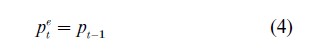
Once this is substituted into Eqn. (3) one obtains p_t=µ+αp_t−1+η_t, which is a stochastic process known as an autoregressive process of first order (AR(1)). This and related stochastic processes are studied in standard textbooks on time series analysis and econometrics.

In the early literature there were no random shocks, yielding a simple difference equation p_t=µ+αp_t−1. This immediately led to the question of whether the generated sequence of prices converged to the stationary state over time. The convergence condition is, of course, |α|<1. Whether this is satisfied depends on the relative slopes of the demand and supply curves. In the stochastic case this condition determines whether the price converges to a stationary stochastic process. (Loosely speaking, a stationary stochastic process is a non-explosive process with statistical properties that are unchanging over time.)

2.2 Adaptive Expectations

The origins of the Adaptive expectations hypothesis can be traced back to Irving Fisher. It was formally introduced in the 1950s by Phillip Cagan, Milton Friedman, and Marc Nerlove. In terms of the price level the hypothesis takes the form

For the cobweb model it can be shown that both expectations and prices converge to stationary stochastic processes, provided the stability condition |1-λ(1-α)|<1 is met.

Adaptive expectations can equivalently be written as a distributed lag with weights declining exponentially at rate 1-λ. Besides adaptive expectations other distributed lag formulations were used in the literature to allow for extrapolative or regressive elements.

Adaptive expectations played a prominent role in macroeconomics in the 1960s and 1970s. For example, inflation expectations were often modeled adaptively in the analysis of the expectations augmented Phillips curve.

3. Rational Expectations

The RE revolution begins with the observations that adaptive expectations, or any other fixed weight distributed lag equation, may provide poor forecasts in certain contexts and that better forecast rules may be readily available. The optimal forecast method depends on the stochastic process of the variable being forecast and this implies interdependency between the forecasting method and the economic model. On this approach we write

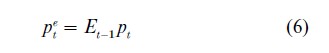
for the cobweb example. E_t−1p_t denotes the mathematical expectation of p_t conditional on variables observable at time t-1 (including past data).

RE is an equilibrium concept. The actual stochastic process followed by prices depends on the forecast rules used by agents, so that the optimal choice of the forecast rule by any agent is conditional on the choices of others. An RE equilibrium imposes the consistency condition that each agent’s choice is a best response to the choices by others. In the simplest models we have representative agents and these choices are identical.

For the cobweb model we have p_t=µ+αE_t−1p_t+η_t. Taking conditional expectations E_t−1 of both sides yields E_t−1 p_t=µ+αE_t−1p_t so that expectations are given by E_t−1p_t=(1-α)⁻¹µ and we have p_t=(1-α)⁻¹ µ+η_t. This is the unique way to form expectations which are ‘rational’ in the model (3).

Two related observations should be made. First, under RE the appropriate way to form expectations depends on the stochastic process followed by the exogenous variables, η_t in the example. If these are not iid processes then the RE will themselves be random variables, and they often form a complicated stochastic process. Second, neither static nor adaptive expectations are in general rational, except in special cases.

Next, we consider some key aspects of RE models.

3.1 Forward-Looking Character

In the cobweb model expectations pertain only to current prices. Most economic models have forward-looking elements, so that expectations about future periods appear. A simple example is the Cagan model of inflation which postulates that the demand for money depends linearly on expected inflation:

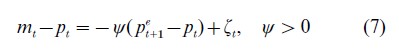
where m_t is the log of the money supply at time t, ζ_t is an iid money demand shock with zero mean, p_t is the log of the price level at time t, and p^e_t+1 denotes the expectation of p_t+1 formed in time t. Solving for p_t we obtain the equation

where α=ψ(1+ψ)⁻, β=(1+ψ)⁻¹, and v_t =-(1+ψ)⁻¹ζ_t. Note that 0<α<1 and β=1-α.

The same formal model arises in other contexts, e.g., the standard model of asset pricing with risk neutrality takes the form of Eqn. (8) with different values for α and β. Under RE the model is

Assume that m_t follows some general exogenous stochastic process. One can show that the expression

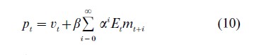
solves the model, provided that the sum converges. Given an exogenous stochastic process for m_t, techniques are available for computing the forecasts E_tm_t+i and hence the RE solution (10).

An important feature of the solution (10) is its forward-looking character. The current price level is a sum of expected values of future money stocks. If, for example, there is a change in monetary policy which is anticipated to lower the money stock from some specified future date T>t, this will be reflected in the price level already at time t. Previously unexpected changes in policy will affect p_t from the moment they become known.

3.2 Solutions To Linear RE Models

Equation (9) is a simple example of a linear RE model. More general models allow for a dependence on lagged values of the endogenous variable p_t, expectations formed at different times and over various horizons, and more general exogenous processes. Generalizations to multivariate frameworks are particularly important in practice.

A number of techniques are available for obtaining solutions under RE. Undetermined coefficient methods are often particularly convenient. Frequently, as in the model (9) with |α|<1, there is a unique nonexplosive solution, given nonexplosive exogenous variables. In this case a method called the Blanchard–Kahn technique can be used to compute this solution.

4. Econometric Issues With Rational Expectations

4.1 Testing For Rationality

If the RE hypothesis is correct, then expectations obey very strong assumptions. The law of mathematical conditional expectations, from probability theory, states that E(E(p|I)|S)=E( p|S) if S and I are alternative information sets with SCI. Here E(p|Ω) denotes the mathematical expectation of p conditional on an information set Ω. This result immediately implies E(e|S)=0, where e=p-E( p|I ).

This result, called the orthogonality principle, implies that the RE forecast error e must be uncorrelated with every variable in the information set.

If data on expectations, for example from surveys, are available, then this provides a straightforward way to test for rationality. Suppose we have time series data on, say, the average one-period ahead forecast f_t of p_t, where the forecast f_t is made based on I_t−1, the information available at time t-1. Under RE f_t E(p_t|I_t−1) and we therefore test whether E(e_t |I_t−1) 0, where e_t =p_t-f_t. In practice, the test is implemented by a regression:

where z_t−1 is a vector of variables in I_t−1. Under the null hypothesis of RE the restrictions H₀: φ=0 hold and u_t is serially uncorrelated. H₀ can be tested using the standard F-test under some additional assumptions. The intuition for the tests is straightforward. If φ ≠0 then forecast errors are systematically correlated with z_t−1 and the information in z_t−1 is not being fully exploited.

Tests can also be conducted using forecast data with multiple period horizons and/or panel data, although these lead to econometric complications. In practice, tests of rationality using survey data on forecasts typically lead to rejections of rationality, although the interpretation of these results is controversial. Supporters of RE often argue that the individuals surveyed are not the relevant group of agents or that the expectations are measured with error. However, rejections of rationality also raise the possibility that agents do deviate from full RE owing to learning, forecasting costs, and/or strategic uncertainty. See Pesaran (1987) for further discussion of econometric tests of the rational expectations hypothesis.

4.2 The Lucas Critique

During the 1950s and 1960s, applied macroeconometric models explicitly or implicitly assumed that expectations were given by adaptive expectations or by some related lag scheme. The estimated systems were used for policy analysis by evaluating the effects of alternative policies. This implicitly assumed that the estimated coefficients reflect a structure that is invariant to alternative policies. Lucas (1976) criticized this approach, arguing that if expectations are rational, then the coefficients relating target variables to policy instruments will change when the policy process changes.

As an example, consider the Cagan model (9) with β=1-α and assume that money supply follows the rule

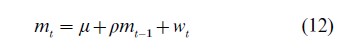
where |ρ|<1 and w_t is an (unforecastable) mean zero iid shock. In this case the solution (10) reduces to

where

The ‘traditional’ approach to policy would estimate δ and γ from historical data and use the estimated version of Eqn. (13) to evaluate the effects of alternative policy sequences m_t on the price level. However, it is clear from Eqn. (14) that γ is not invariant to the policy rule since, for example, a change in the policy parameter ρ affects the value of γ. Thus, under RE, the response of target variables to policy variables depends on the form of the policy rule.

The effect of the ‘Lucas critique’ has been to shift attention to estimation of deep parameters (such as α in the above example), which do remain invariant to policy changes and to use these estimates to evaluate alternative policy rules under RE.

4.3 Estimation And Testing Of RE Models

When data on expectations are not available, it is still often possible in the context of structural models to both estimate the models under the assumption of RE and to test the RE assumption. In this case the RE assumption is being tested jointly with the model. A simple example is the Cagan model (9), with β=1-α, together with the money supply rule (12). Equations (12) and (13) can both be estimated, but Eqns (14a,b) imply that there are nonlinear cross-equation parameter restrictions that are imposed by the RE hypothesis. The system can be estimated under these over identifying restrictions. The restrictions can also be statistically tested, in effect testing RE jointly with the model.

Another strand that has arisen recently is the estimation and testing of Euler equations. These are dynamic equations, relating, e.g., current consumption to expected future consumption and interest rates, which arise as optimality conditions from dynamic utility maximization. Under RE testable over identifying restrictions again arise.

5. Multiple Equilibria And RE

Many RE models can have multiple equilibria. The existence of rational speculative bubble solutions besides the fundamental equilibrium illustrates this phenomenon. The standard model of asset pricing is formally identical with the Cagan model (8) if we set v_t =0, β=1, α=(1+r)⁻¹ , where r is the real net interest rate. Here m_t represents the dividend at t and p_t is the price of the asset. Then Eqn. (10) is called the ‘fundamental solution,’ i.e., the present value of anticipated future dividends. A ‘rational bubble solution’ is the sum of the fundamental solution and a bubble, which is any process B_t satisfying E_tB_t+1 α^-1 B_t. The bubble solutions are ‘explosive’ since α<1, and macroeconomists are often content to assume away ‘explosive bubbles,’ although rational bubbles that burst periodically can be constructed. In models with carefully elaborated microfoundations, explosive solutions can often be ruled out theoretically. Nonetheless, the empirical issue of whether rational (or almost rational) bubbles affect asset prices is still debated.

Other models have multiple RE solutions, none of which are explosive. As a simple example, consider the model p_t =αE_t p_t+1 +βm_t +v_t with |α|>1. (This case can arise from linearized versions of the overlapping generations model of money under some specifications of preferences.) If m_t is iid with mean m, from Eqn. (10) there is the RE solution p_t = (1-α)^-1αβm+βm_t +v_t. However, there are also solutions of the form

where ε_t is an arbitrary process, observable at time t and satisfying E_t−1 (ε_t)=0.

These solutions are well-behaved nonexplosive processes. The variable ε_t is often called a ‘sunspot’ variable and the corresponding equilibrium a ‘sunspot solution.’ The term sunspot is used to indicate the arbitrary nature of the variable. The solution depends on ε_t only because everyone believes that it does. It does not appear in the basic model structure. Guesnerie and Woodford (1992) provide a review of the results on sunspot equilibria and endogenous fluctuations.

It has been demonstrated formally that sunspot solutions can exist in overlapping generations models in which the microfoundations are carefully constructed. More recently it has been shown that, with increasing returns to scale and monopolistic competition, sunspot solutions can exist in variations of common business cycle models. These models raise the possibility that business cycle fluctuations may be due to random but rational fluctuations in household and firm expectations as a ‘self-fulfilling prophecy.’ The empirical significance of self-fulfilling prophecies remains an open issue.

There are numerous other examples of multiple equilibria under RE. One example is provided by a variation of the Cagan model p_t =αE_t p_t+1 +βm_t, where now money supply is assumed to follow a feedback rule m_t =m+ξp_t−1 + u_t. (Here also for convenience v_t =0). This leads to the equation

For many parameter values this equation yields two RE solutions of the form

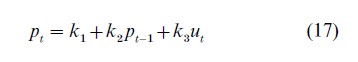
where the k_i depend on the original parameters α, β, ξ, m. In some cases both of these solutions are stochastically stationary.

Other types of multiplicity of RE solutions arise in nonlinear models. Many nonlinear models can be put in the general form

where random shocks have here been left out for simplicity. If y_t is increasing in y^e_t+1, i.e., F`>0, there may be multiple steady states that satisfy y =F (y), i.e., that occur at the intersection of the graph of F (.) and the 45º line. This possibility can arise in models with increasing returns to scale in production, externalities, or monopolistic competition. y is often a measure of output or aggregate economic activity and the low steady states represent inefficient ‘coordination failures’ (Cooper 1999). Other specifications of Eqn. (18) have multiple perfect foresight equilibria taking the form of regular cycles in addition to a steady state.

Nonlinear models can also exhibit sunspot equilibria, taking the form of a finite state Markov process. For example, in models with two steady states it can be shown that there are RE solutions, depending on a two-state Markov sunspot process, in which the solution alternates between values close to the perfect foresight steady states.

6. Learning

The RE approach presupposes that economic agents have a great deal of knowledge about the economy. Even in the simple examples, in which RE are constant, computing these constants requires the full knowledge of the structure of the model, the values of the parameters and that the random shock is distributed iid. In empirical work economists, who postulate RE, do not themselves know the parameter values and must estimate them econometrically. A more plausible view of rationality might thus be that the agents also act like statisticians or econometricians when doing the required forecasting. This insight is the starting point of the Adaptive learning approach to modeling expectations formation.

Taking this approach immediately raises the question of its relationship to RE. In many cases learning can provide at least an asymptotic justification for the RE hypothesis. For example, in the cobweb model (3), if agents estimate an unknown constant expected value by computing the sample mean from past prices one can show that expectations will converge over time to the RE value. In more general models convergence to RE can occur if agents use the appropriate econometric functional form and run regressions in the same way that an econometrician might.

Another major advantage of the learning approach arises when there are multiple equilibria. Consider the above example with a monetary feedback rule in which there are two solutions of the form (17). For the pure RE approach this is a conundrum. Which solution should we and the agents choose? Similarly, in nonlinear models of the form y_t= F ( y^e_t+1) with multiple steady states, cyclic solutions or sunspots, one can ask which equilibria are stable under learning. The adaptive learning approach provides answers to all these questions, as discussed in the next section.

Finally, the transition under learning to RE may itself be of interest. The process of learning adds dynamics that are not present under strict rationality and they may be of empirical importance. In the cases just described these dynamics disappear asymptotically. However, there are various situations in which one can expect learning dynamics to remain important over time. For example, if the economy undergoes structural shifts from time to time then agents will need periodically to relearn the relevant stochastic processes.

6.1 Statistical Approach To Learning

In the adaptive learning approach economic agents behave like statisticians or econometricians when forecasting economic variables needed in their decision making. The economy is taken to be in a temporary equilibrium in which the current state of the economy depends on expectations. The learning approach to expectations formation makes the forecast functions and the estimation of their parameters fully explicit. A novel feature of this situation is that the expectations and forecast functions influence future data points.

As an illustration, consider again the cobweb model (3). Assume that agents believe that the stochastic process for the market price takes the form p_t =constant+noise, i.e., the same functional form as the RE solution. The sample mean is the standard way for estimating an unknown constant, and in this example it is also the forecast for the price. Thus agents’ expectations are given by p^e_t =1/t ∑^t-1_t=0 p_i. Combining this with Eqn. (3) leads to a fully specified stochastic dynamic system. It can be shown that the system under learning converges to the RE solution if α<1.

If the economic model incorporates exogenous or lagged endogenous variables, it is natural for the agents to estimate the parameters of the perceived process for the relevant variables by means of least- squares regressions. As an illustration suppose that an observable exogenous variable w_t−1 is introduced into the cobweb model, so that Eqn. (3) now takes the form

It would now be natural to forecast the price as a linear function of the observable w_t−1. In fact, the unique RE solution is of this form:

where a=(1-α)⁻¹μ and b=(1-α)⁻¹ϐ and the corresponding rational forecast is p_t =a+bw_t−1.

Under least-squares learning agents would forecast according to

where a_t−1 and b_t−1 are parameter estimates obtained by a least-squares regression of p_t on w_t−1 and an intercept, using the data available through time t-1.

It can be shown that (a_t, b_t) converges to the unique REE (a, b) if α<1.

6.2 Stability Under Learning

In general, when expectations are modeled by least-squares learning there is convergence to the REE as t→∞ provided that a stability condition is met. The stability condition can usually be obtained by the expectational stability approach.

To illustrate this approach for the cobweb model (19), suppose that expectations are based on the perceived law of motion (PLM) p_t =a+bw_t−1 +η_t and hence given by p^e_t=a+bw_t-1, where (a, b) may not be the REE values. Substituting this into Eqn. (19) we obtain the corresponding actual law of motion (ALM):

This yields a mapping from the PLM parameters (a, b) into the ALM parameters T (a, b)=( µ+αa, δ+αb). Only at the REE values does one have T(a, b)=(a, b). Expectational stability (E-stability) looks at whether the REE is the stable outcome of a process in which the parameters of the PLM are adjusted slowly toward the parameters of the ALM that they induce. Formally, this adjustment is described by a differential equation and E-stability corresponds to local stability of the REE under these dynamics. For details, see Evans and Honkapohja (2001).

In the cobweb model the E-stability condition is given by α<1. Even in fairly complicated models it is often straightforward to compute E-stability conditions and these appear generally to govern convergence of statistical learning rules.

Local stability under adaptive learning, or E-stability, provides a selection criterion in models with multiple RE equilibria. For example, in the Cagan model with policy feedback (16) there are two RE solutions of the form (17), but only one of these is E-stable and hence stable under least-squares learning. The other solution, although rational, is therefore unlikely to arise in practice. Similarly, in the nonlinear model y_t =F ( y^e_t+1), only the steady states with slope F( y)<1 are E-stable. This model can also have sunspot solutions and it has been shown that an appropriate form of adaptive learning can converge to rational sunspot equilibria, provided the corresponding E-stability condition is satisfied.

6.3 Other Approaches To Learning

There are some other recent approaches to modeling expectation formation. ‘Educti e learning’ and‘rational learning’ are closer to RE than adaptive learning. In the former agents engage in a process of reasoning using common-knowledge assumptions and the learning takes place in logical or notional time. Rational learning takes place in real time, but retains the RE equilibrium assumptions at each point in time.

In contrast, the adaptive learning approach assumes that agents possess a form of bounded rationality which may, however, approach rational expectations over time. Besides the statistical formulation outlined above, alternative models of bounded rationality learning have been studied. Concepts from computational intelligence, such as genetic algorithms, neural networks and classifier systems, have been used as models of adaptive learning in economics.

Finally, we note that the literature has also considered learning in situations with structural shifts and/or misspecification of the perceived stochastic process. Certain learning rules, such as constant gain algorithms, can track structural changes more accurately than least-squares algorithms, although they often fail to converge fully to an RE equilibrium if the economic structure is in fact constant. Such procedures can lead to new forms of persistent learning dynamics which may be empirically important.

Bibliography:

1. Cooper R 1999 Coordination Games, Complementarities and Macroeconomics. Cambridge University Press, Cambridge, UK
2. Evans G W, Honkapohja S 2001 Learning and Expectations in Macroeconomics. Princeton University Press, Princeton, NJ
3. Farmer R E 1999 The Economics of Self-fulfilling Prophesies, 2nd edn. MIT Press, Cambridge, MA
4. Guesnerie R, Woodford M 1992 Endogenous fluctuations. In: Laffont J-J (ed.) Advances In Economic Theory: Sixth World Congress. Cambridge University Press, Cambridge, UK, Vol. 2
5. Keynes J M 1936 The General Theory of Employment, Interest and Money. Macmillan, London
6. Lucas R E Jr 1976 Econometric policy evaluation: A critique. In: Lucas R E Jr (ed.) Studies in Business Cycle Theory. MIT Press, Cambridge, MA (originally published in 1976)
7. Lucas R E Jr 1981 Studies in Business Cycle Theory. MIT Press, Cambridge, MA
8. Lucas R E Jr, Sargent T J (eds.) 1981 Rational Expectations and Econometric Practice. University of Minnesota Press, Minneapolis, MN
9. Muth J F 1961 Rational expectations and the theory of price movements. Econometrica 29: 315–35
10. Pesaran M H 1987 The Limits to Rational Expectations. Blackwell, Oxford, UK
11. Sargent T J 1987 Macroeconomic Theory, 2nd edn. Academic Press, New York