Economic Panel Data Research Paper

The increasing popularity of panel studies is partly a consequence of more cost effective ways of developing and maintaining panels (e.g., Matyas and Sevestre 1996). More importantly, panel data offers many more possibilities for exploring analytical and substantive issues than purely cross-sectional or time series data. However, new data sources also raise new issues. This research paper reviews the major advantages and limitations of panel data in the context of specific econometric methodologies. Section 2 gives an overview of the major advantages of the informational content of panel data. Section 3 reviews typical specifications for the linear models. Section 4 discusses issues of nonlinear models. Section 5 considers the implication of sample attrition and sample selection. Conclusions are in Sect. 6.

2. Advantages Of Panel Data

Panel data offer several advantages over a single cross-sectional or time series data. For instance, the use of panel data may:

2.1 Improve The Accuracy Of Parameter Estimates

Most statistical estimators converge to the true parameters at the speed of the square root of the degrees of freedom. Models for panel data are based on many more equivalent observations than a cross-sectional or time series data, and hence can yield more accurate parameter estimates.

2.2 Lessen The Problem Of Multicollinearity

Many economic variables tend to move collinearly over time. The shortage of degrees of freedom and severe multicollinearity problems found in time series data often frustrate investigators who wish to determine the individual influences of each explanatory variable. Panel data may lessen the degree of multicollinearity in the time dimension by appealing to inter-individual differences.

2.3 Allow The Specification Of More Complicated Behavioral Hypotheses

A single time series is not useful for discriminating hypotheses which depend on different social–demographic factors. Cross-sectional data cannot be used to model dynamics. Cross-sectional data can show what proportion of the labor force is unemployed or describe the distribution of wage rates at a point in time. Aggregate time series data can provide indications of general trends and cyclical patterns in unemployment, wages, income, and so forth. But neither cross-sectional nor time series data can provide information regarding how many of those unemployed in one month can find employment in the next month. Neither can the data provide information on whether the tendency of welfare families to stay on welfare occurs simply because the same factors that cause them to be on welfare keep them there or whether, in addition, the experience of receiving welfare has some addictive effect that induces continuing welfare dependence. For instance, suppose that a cross-sectional sample of married women is found to have an average yearly labor force participation rate of 50 percent. At one extreme this might be interpreted as implying that each woman in a homogenous population has a 50 percent chance of being in the labor force in any given year while at the other extreme it might imply that 50 percent of the women in a heterogenous population always work and 50 percent never work. In the first case, each woman would be expected to spend half of her married life in the labor force, and half out of the labor force, and job turnover would be expected to be frequent, with an average job duration of two years. In the second case, there is no turnover, and current information about work status is a perfect predictor of future work status. Panel data, by providing sequential observations for a number of individuals, offer the possibility to distinguish inter-individual differences from intra-individual dynamics and to construct a proper recursive structure to study the effects of changes by comparing the differences before and after the changes (e.g., Heckman 1981).

2.4 Pro Ide Possibilities For Reducing Estimation Bias

A standard assumption in statistical specification is that the random error term representing the effect of omitted variables is orthogonal to the included explanatory variables. Otherwise, the estimates are subject to omitted variable bias when these correlations are not explicitly allowed for. Panel data provide means to eliminate or reduce the omitted variable bias through various data transformations when the correlations between included explanatory variables and omitted variables follow certain specific patterns (e.g., Baltagi 1995), Chamberlain 1984, Hsiao (1986). For instance, suppose that

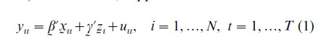
where the explanatory variables x_it, vary across individuals i, and over time t, and the explanatory variables z_i, vary across i, but stay constant over t, such as sex status, social-demographic background variables, etc. the error term u is assumed to be uncorrelated with x or z. The least squares regression of y on x and z will yield consistent estimates of β and γ. But if z are correlated with x, yet are unobservable, the least squares regression of y on x will yield bias estimates of β. However, in the pairwise difference,

the explanatory variables z_i longer enter. Regressing ( y_it-y_{i, t−1} ) on (x_it-x_{i, t−1}) can yield consistent estimates of β.

MaCurdy’s (1981) life-cycle labor supply of primeage males under certainty is an example of this approach. Under certain simplifying assumptions, MaCurdy shows that a worker’s labor supply function can be written as in Eqn. (1), where y is the logarithm of hours worked, x is the logarithm of the real wage rate, and z is the logarithm of the worker’s (unobserved) marginal utility of initial wealth, which, as a summary measure of worker’s lifetime wages and property income, is assumed to stay constant through time but to vary across individuals. Given the economic problem, not only is x_it correlated with z_i, but every economic variable that could act as an instrument for x_it (such as education) is also correlated with z_i. Another example is the ‘conditional convergence’ of the growth rate. The growth rate regression model typically includes investment ratio, initial income, and measures of policy outcomes like school enrolment and the black market exchange rate premium as regressors; however, an important component, the initial level of a country’s technical efficiency z_i0 , is not observed. Since a country that is less efficient is also more likely to have lower investment rate or school enrolment, one can easily imagine that z_i0 is correlated with the included repressors. Neither model can be estimated with cross-sectional data, but both can be estimated using Eqn. (2) if panel data are available.

2.5 Reduce Computational Complexities

The use of panel data is often perceived as increasing computational complexities because the data contain both cross-sectional and time series dimensions. In many cases, however, panel data become a distinct advantage computationally. For instance, if one were to estimate a dynamic model using time series data with censored or missing observations in between, the computation can be horrendous because of the need to compute multiple integrals when the conditional variables are censored. To see this, consider the model

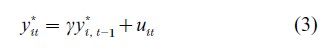
where u_it is independent normal with mean 0 and variance σ_u². Conditional on y*_t,i-1, y*_u is normally distributed with mean γy*_t,i-1 and variance σ_u. If instead of observing y*_it , however, one observes the censored counterpart y_it, where y_it=y*_it if y*_it>0 and y_it=0 if y*_it≤0, then the conditional distribution of y_it given y_{i, t−1} 0 becomes

where f( y*_I,t-1) denotes the marginal density of (y*_I,t-1).

When there are a number of censored observations over time, Eqn. (4) becomes relatively complicated to solve. With panel data, one can often adopt models that ignore observations that are censored and focus on those individuals for which successive observations are greater than zero to simplify the computation (e.g., Arellano et al. 1999).

2.6 Simplify Statistical Inference

In estimating a dynamic model using time series, the limiting distribution depends on whether the system is stable, integrated, or explosive. With panel data, as long as the cross-sectional dimension approaches infinity, the limiting distribution of the coefficients of lagged dependent variables is typically normal no matter what the time series properties of a process are. The limiting distribution remains the same whether the time series dimension is fixed (Anderson and Hsiao 1982) or approaches infinity (Levin and Lin 1993, Phillips and Moon 1999).

2.7 Obtain More Accurate Prediction Of Individual Outcomes

When people’s behavior is similar in nature, namely, they satisfy De Finnetti’s (1964) exchangeability assumption, each individual’s behavior can be better understood by observing the behavior of other similar individuals, hence can yield more accurate predictions of individual outcomes by pooling the data (e.g., Hsiao et al. 1989).

3. Linear Models

Panel data, by its nature, put emphasis on individual outcomes. Different individuals may be subject to different influences. In explaining individual behavior, one may extend the list of factors ad infinitum. It is neither feasible nor desirable to include all the factors affecting the outcome of all different individuals in a model specification. It is typical to leave out those factors that are believed to have insignificant impact or are peculiar to a given individual. However, when important factors peculiar to a given individual are left out, the individual outcomes conditional on the included explanatory variables may not be viewed as random draws from a common population, so standard statistical procedures may mislead. Therefore, one focus of panel data modeling is to determine whether heterogeneities exist among cross-sectional units over time that are not captured by the included explanatory variables, say x. If they are, one needs to control the impact of such unobserved heterogeneity in order to draw inference about the population characteristics.

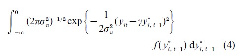
If the unobserved heterogeneity among N cross- sectional units over T time periods can not be completely captured by x, there are two primary ways to model it. One is to incorporate it into the error term. The other is to let the coefficients vary across individuals and over time. For instance, if the heterogeneity among individual units is due to some individual specific and time invariant variables, z_i, that affect y_it linearly, then the scatter diagram between y and x conditional on z may look like Fig. 1 in which the broken-line circles represent the point scatter for an individual over time, and the broken straightline represents the mean relationship for the ith individual conditional on z_i. The dark line indicates a simple pooled estimates of a model

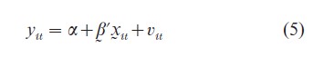
where v represents the effects of omitted factors and the subscript, it, indicates observations of the ith cross-sectional unit at tth time period. It is obvious that the simple pooled estimates give a very misleading relationship between y and x. For data of the form of Fig. 1 it is necessary to specify a variable intercept model of the form

where α_i represents the effect of unobserved z_i.

A more complicated structure to capture the unobserved heterogeneity lets

but this specification is not very useful for drawing inferences about the population because the coefficients are individual and time specific. Neither can it be estimated because there are more unknown parameters than degrees of freedom. In order to take advantage of panel data, a structure has to be introduced that allows the possibility to draw inference about the population characteristics while controlling for the impact of unobserved heterogeneity.

Suppose that the unobserved heterogeneity is due to some individual specific but time invariant variables, then an unrestricted linear model will have the form

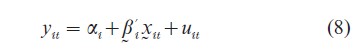
If T is large, Eqn. (8) can be estimated by Zellner’s (1962) seemingly unrelated regression method; however, most panel data contains a large number of individuals observed over a short period of time. When T is fixed, increasing N increases the number of unknown parameters, α_i and β_i, i=1, …, N. This is the classical incidental parameter problem. The presence of the incidental parameters violates the usual regularity conditions for the consistency of the maximum likelihood estimator (MLE). Neither is Eqn. 3.4 very useful to draw inference about the population because each individual has a different behavioral pattern. Assuming Eqn. (8) is tantamount to assuming that the cross-sectional observations come from heterogeneous population. In this case there is no particularly appealing reason to pool the data.

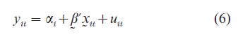
To draw inference about the population, one must impose restrictions on Eqn. (7) or Eqn. (8). For instance, if the slope coefficients are the same, β_i=β, for all i as in Eqn. (6), the incidental parameter αi can be eliminated by pairwise differencing of individual time series observations as in Eqn. 2 or by taking deviations from the individual time series mean:

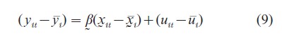
where y_i=(1/T ) ∑^T_t=₁y_u,x₁=(1/T)∑^T_t=1x_u and u_t=(1/T)∑^T_t=1u_it. Applying the least squares method to Eqn. (9) yields the so-called covariance or within estimator of β. The covariance estimator of β is consistent when either N or T or both N and T tend to infinity (e.g., Hsiao 1986).

Alternatively, one can assume that β_i and/or α_i in Eqn. (8) are randomly distributed with common mean (β , α) and covariance matrix ∆ or assume that some of the coefficients are randomly distributed with common mean and constant covariance matrix, while others are fixed and different. Decomposing x_it into (w_it, z_it), various formulations can be represented as placing different restrictions on the unconstrained model Eqn. (8):

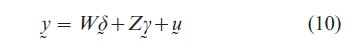
where y=( y`<sub>1</sub>, …, y`_N), W=diag(W_i), Z=diag (Z_i), y_i=( y_i1 , …, y_iT)`, W<sub>i</sub> and Z<sub>i</sub> are T×k<sub>1</sub> and T×k<sub>2</sub> submatrices of T observed values of (1, x`_it), δ = (δ₁, …, δ _N)` and γ=(γ₁, …, γ_N) are Nk₁×1 and Nk₂×1 vectors of (α_i, β_i), i=1, …, N. Suppose that the coefficients of w_it are subject to stochastic constraints:

where A₁ is an N_k1×m matrix with known elements, δ is an m×1 vector of constants, ε is random with mean 0, covariance matrix C and E_εW`=0, EεZ`=0. Suppose that the coefficients of z_it are subject to deterministic constraints:

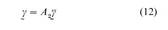
where A₂ is an N_k2×q matrix with known elements, and γ is a q×1 vector of constants.

The model given by Eqns. (10)–(12) is of a mixed form: the coefficients of Wi are assumed to be random and the coefficients of Z_i are assumed fixed, (e.g., Hsiao and Tahmiscioglu 1997). When W=0, A₂=e_N ϱΘI_k , we have a common model for all NT observations, where e_N denotes an N×1 vector of ones, I_p denotes a p×p identity matrix and denotes Kronecker product. When W=0 and A=I_Nk , model Eqn. (8) results. when W=0, Z_i =(e_T, X_i), A₂= (I_NΘi_k2:e_NΘI*_k2-1) is a k₂×1 vector of (1, 0, …, 0)’’, and I*_k2-1 is a k₂ ×(k₂-1) matrix of (I⁰_k2-1), model Eqn. (6) (e.g., Mundlak 1978) is a special case. When X_i=e_T, A₁=e_N, ∆=σ²δ I_N, the model is the error components model (e.g., Balestra and Nerlove 1966). Finally when Z=0, A₁=e_NΘI_k , C=I_NΘ∆, we have the random coefficients model (e.g., Swamy 1970).

Substituting Eqns. (11) and (12) into Eqn. (10) yields

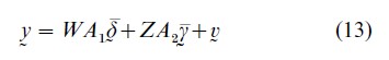
where v=Wε+u, Evv`=WCW`+Cov (u). Model Eqn. (13) can be estimated by the generalized least squares (GLS) method. The individual coefficients δ can be estimated by a Bayes estimator which is a weighted average of the GLS estimator of δ and the individual least squares estimator of δ (e.g., Hsiao et al. 1993).

The issue of whether to treat β_i and/or α_i or a subvector of them as fixed or random is an issue of whether conditional on x, one can treat the outcome variable as a random draw from a common population. If it is, then the individual and time subscript, it, can be viewed as purely a labeling device and a priori, E (y_it|x)=E (y_js|x). This is what de Finnetti (1964) called the exchangeability criterion and it is more appropriate to treat β_i and α_i as random. If the distribution of β_i is not independent of x_it or conditional on x, individual outcomes are more appropriately viewed as generated from a heterogenous population, then the subscript, it, contains specific information about which heterogenous population the particular observation is generated from. It is therefore more appropriate to treat β_i and/or α_i as fixed parameters. Unfortunately, a priori, very little knowledge is available about which coefficients should be treated as random and different, and which coefficients should be treated as fixed and different. Hsiao and Sun (2000) have argued that the random versus fixed effects specification should be viewed as a model selection issue and suggest a Bayesian approach for model selection. Their limited Monte Carlo studies appear to favor the Schwarz (1978) information criterion to select the appropriate specifications. The Schwarz criterion works here because although from a Bayesian perspective there is no real difference between random effects and fixed effects since every parameter has a distribution, there is a difference between how the prior is formulated under the random and fixed effects formulation. Under the di Finnetti exchangeability criterion, β_i is distributed independently of x_i with a common mean β and constant variance C (e.g., Eqn. (11)). On the other hand, under the fixed effects formulation, each β_i is supposed to be independently distributed with a different mean and different variance because of the correlation between β_i and x_i or because each β_i is a random draw from heterogenous population.

4. Nonlinear Models

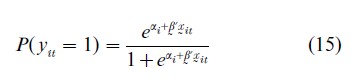
The estimation of a nonlinear panel data model involving individual specific effects is particularly difficult to handle. If the individual specific effects are treated as random, just as in the linear model, we no longer have the incidental parameters problem; however, the estimation of the structural parameters requires integrating out the individual specific effects which can be nontrivial. For instance, consider a binary choice model in which y_it takes the value of either 1 or 0. Suppose that the probability of observing y_it=1, P (y_it=1|x_it), is given by F (β x_it +α_i), where the individual specific effects αi is randomly distributed with density function f (α_i). Even though conditional on α_i , y_it may be independently distributed over i and t, unconditionally, y_it is correlated over T. The log-likelihood function is of the form

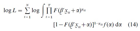
Equation (14) is a function of finite number of parameters and maximizing it under weak regularity conditions will yield consistent estimator of β (and the parameters characterizing the density function of α_i). However, maximizing (Eqn. (14)) is often computationally infeasible. For instance, if F (·) takes the form of an integrated standard normal distribution function, then a probit model results. Conditional on α_i, it involves a univariate integration. Maximizing (Eqn. (14)) but without the conditioning involves the evaluation of T-dimensional integrals (e.g., Hsiao 1986).

On the other hand, suppose that the individual specific effects are fixed. First, in general there is no simple transformation of the data as in Eqns. (2) or (9) to eliminate the individual specific effects (incidental parameters). Second, the estimation of the individual specific parameters and the structural (or common) parameters are not independent of each other. When a panel contains a large number of individuals but only over a short time period, the error in the estimation of the individual specific coefficients propagates into the estimating of the structural parameters, and hence leads to inconsistency of the structural parameter estimation (e.g., Anderson and Hsiao 1982).

Many approaches have been suggested for estimating fixed effects nonlinear panel data models. One approach is by conditioning the likelihood function on the minimum sufficient statistics for the incidental parameters to eliminate the individual specific parameters (Andersen 1973, Chamberlain 1980). For instance, consider a binary logit model in which the probability of y_it=1 is given by

For ease of exposition, assume that T=2. It can be shown that when x_i =0 and x_i=1 the MLE of β converges to 2β as N→∞, which is not consistent (e.g., Hsiao 1986). However, one may condition the likelihood function on the minimal sufficient statistic for α_i. We note that those individuals i satisfying y_i1 +y_i2 =2 or y_i1+y_i2=0 provide no information about β since the former leads to α_i=∞ and the latter leads to α_i=-∞. Hence one can concentrate on those individuals with y_i1+y_i2=1. For those individuals satisfying y_i1+y_i2=1, let d_i=1 if y_i1=0 and y_i2=1 and d_i=0 if y_i1=1 and y_i2=0. Then

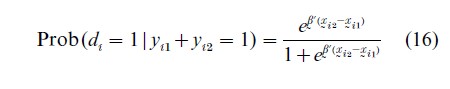
Eqn. (16) no longer contains the individual effects α_i and is of the form of a standard logit model. Therefore, maximizing the conditional log-likelihood function on the subset of individuals with y_i1+y_i2=1 is consistent and asymptotically normally distributed.

Alternatively, one can transform the data to eliminate the individual effects if the nonlinear model has a latent linear structure, and then apply semiparametric methods. For instance, consider a binary choice model with y_it =1 if y*_i1>0 and y_it=0 if y*_i1≤ 0, where

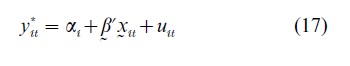
If u_it follows a logistic distribution, a logit model results; if uit is normally distributed, a probit model results. Then

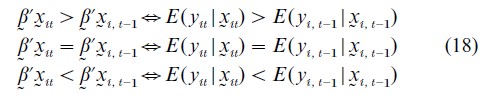
Rewriting (Eqn. (18)) into the equivalent first difference form, Manski (1975) proposes a maximum score estimator (MS) that maximizes the sample average function

where sgn [(x_it-x_{i, t−1})`β ]=1 if (x<sub>it</sub> -x<sub>i, t−1</sub> )`β≥0 and sgn [(x_it-x_{i, t−1} )`β ]=-1 if (x_it-x_{i, t−1} )β<0. The MS estimator is consistent but is not root-n consistent, where n=N (T-1). Its rate of convergence is n^1/3 and n^1/3(β-β) converges to a random variable that maximizes a certain Gaussian process.

A third approach is to find an orthogonal reparameterization of the fixed effects for each individual, say α_i, to a new fixed effects, say g_i, which are independent of the structural parameters in the information matrix sense. The g_i are then integrated out of the likelihood with respect to an uninformative, uniform prior distribution which is independent of the prior distribution of the structural parameters. Lancaster (2001) uses a two period duration model to show that the marginal posterior density of the structural parameter possesses a mode which consistently estimates the true parameter.

While all these methods are quite ingenious, unfortunately, none can claim general applicability. For instance, the conditional maximum likelihood cannot work for the probit model because there are no minimal sufficient statistics for the incidental parameters that are independent of the structural parameters. The data transformation approach cannot work if the model does not have a latent linear structure. The orthogonal reparameterization approach works only for particular models. In short, the methodology for and consistency of nonlinear panel data estimators must be established case by case.

5. Sample Attrition And Sample Selection

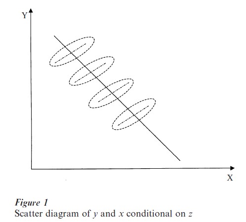
Missing observations occur frequently in panel data. If individuals are missing randomly, most estimation methods for the balanced panel can be extended in a straightforward manner to the unbalanced panel (e.g., Hsiao 1986). For instance, suppose that

where d_it is an observable scalar indicator variable which denotes whether information about ( y_it, x_it`) for the ith individual at tth time period is available or not. The indicator variable d_it is assumed to depend on a q- dimensional variables, wit, individual specific effects λ_i and an unobservable error term η_it,

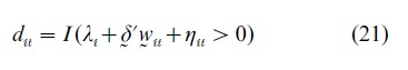
where I (·) is the indicator function that takes the value of 1 if λ_i+δ`w_it+η_it>0 and 0 otherwise. In other words, the indicator variable d_it determines whether ( y_it, x_it)) in Eqn. (20) is observed or not.

Without sample selectivity, that is d_it=1 for all I and t, Eqn. (20) is the standard variable intercept (or fixed effects) model for panel data discussed in Sect. 2. With sample selection and if η_it and u_it are correlated, E(u_it|x_it, d_it =1)≠0. Let θ(·) denote the conditional expectation of u_it conditional on d_it=1 and x_it, then Eqn. (20) can be written as

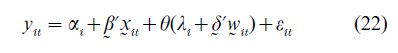
where E (ε_it|x_it, d_it=1)=0. The form of the selection function is derived from the joint distribution of u and η. For instance, if u and η are bivariate normal, then we have the Heckman (1979) sample selection model with

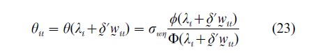
where σ_wη denotes the covariance between w and η, φ(·) and Φ(·) are integrated standard normal density and distribution, respectively and the variance of η is normalized to be 1. Therefore, in the presence of sample attrition or selection, regressing y_it on x_it using only the observed information is invalidated by two problems—first, the presence of the unobserved effects α_i, and second, the ‘selection bias’ arising from the fact that E (u_it|x_it, d_it=1)=θ(λ_i+δw_it).

When individual effects are random and the joint distribution function of (u, η, γ_i, λ_i) is known, both maximum likelihood and two or multi-step estimators can be derived (e.g., Heckman 1979). The resulting estimators are consistent and asymptotically normally distributed. The speed of convergence is proportional to the square root of the sample size. However, if the joint distribution of u and η is mis-specified, then even without the presence of α_i, both the maximum likelihood and Heckman (1979) two step estimators are inconsistent. This sensitivity of parameter estimate to the exact specification of the error distribution has motivated interest in semiparametric methods.

The individual specific effects in Eqn. (20) are easily eliminated by time differencing for those individuals that are observed for two time periods t and s, i.e., those individuals i satisfying d_it=d_is=1. However, the sample selectivity factors are not eliminated by time differencing. Ahn and Powell (1993) note that if θ is a sufficiently ‘smooth’ function, and δ is a consistent estimator of δ, observations for which the difference (w_it -w) δ is close to zero should have θ_it-θ_is ≈0. They propose a two-step procedure. In the first step, consistent semiparametric estimates of the coefficients of the ‘selection’ equation are obtained. The result is used to obtain estimates of the ‘single index, w_itδ,’ variables characterizing the selectivity bias in the index equation. The second step of the approach estimates the parameters of the equation of interest by a weighted instrumental variables regression of pairwise differences in dependent variables in the sample on the corresponding differences in explanatory variables: the weights put more emphasis on pairs with w_itδ≈w_{i, t−1} δ.

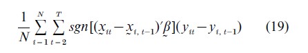
Kyriazidou (1997) generalizes this concept and proposes to estimate the fixed effects sample selection models in two steps: in the first step, estimate δ by either Chamberlain (1980) conditional maximum likelihood approach or the Manski (1975) maximum score method. In the second step, the estimated δ is used to estimate γ, based on pairs of observations for which d_it=d_is=1 and for which (w_it -w_is)`δ is ‘close’ to zero. This last requirement is operationalized by weighting each pair of observations with a weight that depends inversely on the magnitude of (w<sub>it</sub> -w<sub>is</sub>)`δ, so that pairs with larger differences in the selection effects receive less weight in the estimation. The Kyriazidou (1997) estimator takes the form

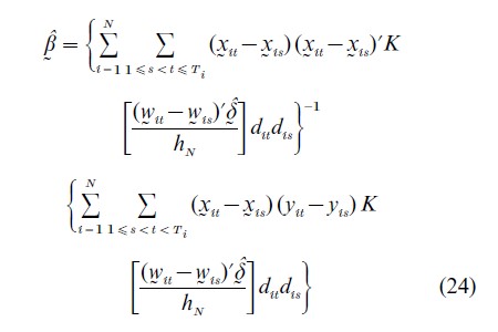
where K is a kernel density function which tends to zero as the magnitude of its argument increases and h_N is a positive constant that decreases to zero as N→∞. Under appropriate regularity conditions, Eqn. (24) is consistent but the rate of convergence is much slower than the standard square root of the sample size.

6. Conclusions

Panel data have opened up avenues of research that simply could not have been pursued otherwise, but their power depends on the extent and reliability of the data as well as on the validity of the restrictions upon which the statistical methods have been built. Otherwise, panel data may provide a solution for one problem, but aggravate another. For instance, consider the income-schooling example given by Griliches (1979):

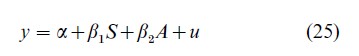
where y is a measure of income, S is a measure of schooling, A is an unmeasured ability variable which is assumed to be positively related to S. If S and A are uncorrelated, the least squares regression of y on S will yield consistent estimates of β₁. If S and A are correlated, then the least squares estimator of β₁ will suffer from omitted variable bias. If A is a purely ‘family’ variable in the sense that siblings have exactly the same level of A, then estimation of β₁ from differences between the brothers’ earnings and differences between the brothers’ education is consistent. But, if ability, apart from having a family component also has an individual component related to the schooling variables, then the within family estimate of β is again biased and the bias is not necessarily less than that of the least squares estimate.

This example demonstrates that the usefulness of panel data in providing particular answers to certain issues depends on the validity of the assumptions implicit in the model. Since there is no universally acceptable way of modeling unobserved heterogeneity in panel data, it would be more fruitful to explicitly recognize the limitations of the data and focus attention on developing models and estimation methods based on what is observable, avoiding imposing arbitrary assumptions on the model and data. For additional discussions on panel data methodology, see Baltagi (1995), Hsiao (1986), and Matayes and Sevestre (1996).

Bibliography:

1. Ahn H, Powell J L 1993 Semiparametric estimation of censored selection models with a nonparametric selection mechanism. Journal of Econometrics 58: 3–80
2. Andersen E B 1973 Conditional Inference and Models for Measuring. Mentalhygrejnisk Forlag, København
3. Anderson T W, Hsiao C 1982 Formulation and estimation of dynamic models using panel data. Journal of Econometrics 18: 47–82
4. Arellano M, Bover O, Labeaga J 1999 Autoregressive models with sample selectivity for panel data. In: Hsiao C, Lahiri K, Lee L F, Pesaran M H (eds.) Analysis of Panels and Limited Dependent Variable Models. Cambridge University Press, Cambridge, UK, pp. 23–48
5. Balestra P, Nerlove M 1966 Pooling cross-section and time series data in the estimation of a dynamic model: the demand for natural gas. Econometrica 34: 585–612
6. Baltagi B H 1995 Econometric Analysis of Panel Data. Wiley, New York
7. Chamberlain G 1980 Analysis of covariance with qualitative data. Review of Economic Studies 47: 225–38
8. Chamberlain G 1984 Panel data. In: Griliches Z, Intriligator M (eds.) Handbook of Econometrics, vol. II. North Holland, Amsterdam, pp. 1247–318
9. De Finnetti B 1964 Farsight: its logical laws, its subjective sources. In: Kyburg H E Jr, Smokler H E (eds.) Studies in Subjective Probability. Wiley, New York, pp. 93–158
10. Griliches Z 1979 Sibling models and data in economics, beginning of a survey. Journal of Political Economy 87: supplement 2, S37–S64
11. Heckman J J 1979 Sample selection bias as a specification error. Econometrica 47: 153–161
12. Heckman J J 1981 Heterogeneity and state dependence. In: Rosen S (ed.) Studies in Labor Markets. Chicago University Press, Chicago, pp. 91–139
13. Hsiao C 1986 Analysis of panel data. Econometric Society monographs No. 11. Cambridge University Press, New York
14. Hsiao C, Appelbee T W, Dineen C R 1993 A general framework for panel data models—with an application to Canadian customer dialled long distance telephone service. Journal of Econometrics 59: 63–86
15. Hsiao C, Mountain D C, Tsui K Y, Luke Chan M W 1989 Modeling: Ontario regional electricity system demand using a mixed fixed and random coefficients approach. Regional Science and Urban Economics 19: 567–87
16. Hsiao C, Sun B 2000 To pool or not to pool panel data. In: Krishnakumar J, Ronchetti E (eds.) Panel Data Econometrics: Future Directions; Papers in Honor of Professor Pietro Balestra. North Holland, Amsterdam, pp. 181–98
17. Hsiao C, Tahmiscioglu A K 1997 A panel analysis of liquidity constraints and firm investment. Journal of American Statistical Association. 92: 455–65
18. Kyriazidou E 1997 Estimation of a panel data sample selection model. Econometrica 65: 1335–64
19. Lancaster T 2001 Some econometrics of scarring. In: Hsiao C, Morimune K, Powell J (eds.) Nonlinear Statistical Modeling: Proceedings of the 13th International Symposium in Economic Theory and Econometrics: Essays in Honor of Takeshi Amemiya. Cambridge University Press, New York, pp. 393–402
20. Levin A, Lin C 1993 Unit Root Tests in Panel Data: Asymptotic and Finite Sample Properties. Department of Economics, University of California, San Diego
21. MaCurdy T E 1981 An empirical model of labor supply in a life cycle setting. Journal of Political Economy 89: 1059–85
22. Manski C F 1975 Maximum score estimation of the stochastic utility model of choice. Journal of Econometrics 3: 205–28
23. Matyas L, Sevestre P (eds.) 1996 The Econometrics of Panel Data—Handbook of Theory and Applications, 2nd edn. Kluwer, Dordrecht, The Netherlands
24. Mundlak Y 1978 Pooling of time series and cross section data. Econometrica 46: 69–85
25. Phillips P C B, Moon H R 1999 Linear regression limit theory for nonstationary Panel Data. Econometrica 67: 1057–111
26. Schwarz G 1978 Estimating the dimension of a model. Annals of Statistics 6: 461–4
27. Swamy P A V B 1970 Efficient inference in a random coefficient regression model. Econometrica 38: 311–23
28. Zellner A 1962 An efficient method of estimating seemingly unrelated regressions and tests for aggregation bias. Journal of American Statistical Association 57: 348–68