Economic Measurement and Forecasting Research Paper

An interested person learning about macroeconomic policy decision making, after reading the preceding paragraph, curiously asks a series of questions focused on identifying economic activities, measuring economic activities, modeling information, economic forecasting, and decision and policy making. The focus of this research paper is to briefly provide answers to some of these questions without getting into the complexities inherent in their details.

A recession is a contraction or downturn in overall economic activity when output and employment decline, generally for a period of 6 months (two quarters) or more. A severe and long contraction is called a depression. A relatively mild and short contraction (less than 6 months) is referred to as a downturn or slowdown. When economic activities change at a positive rate (output and employment are rising), the economy is said to be in an expansion phase. When the demand for the goods and services in an economy exceeds its ability to meet them or when for some other reason prices throughout the economy rise, the economy experiences inflation. Stagflation occurs when an economy experiences high unemployment and inflation simultaneously.

The preceding phases of the economy reflect the business cycle (Figure 1). Each economy has a long-run growth rate that is dependent on its economic structure and a range of socioeconomic and technological factors. In a dynamic economy, as these factors change—for example, through technological advancements—the long-run growth rate will change. In the short run, economic growth may be rising or falling around the long-run growth rate. When the short-run growth rate is falling, the economy is in a slowdown that may lead to a recession. When the short-run growth rate is rising, the economy is in an expansion. These are the phases of the business cycle. A business cycle consists of an expansion and a contraction that follow each other separated by a peak and a trough. A peak, the high point of a cycle, is the beginning of a downturn, and a trough, the low point of a cycle, is the beginning of an expansion. An expansion may contain one or more downturns and slowdowns. Not all the slowdowns and downturns end up in a recession, and predicting if and when a recession will occur is difficult.

Figure 1.   The Business Cycle

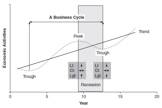
NOTE: A business cycle consists of an expansion and a contraction that follow each other, separated by a peak and a trough. A peak is identified when the changes in leading indicators are negative, no changes are observed in the coincidental indicators, and the changes in the lagging indicators are positive. A trough is identified when the changes in the leading indicators are positive, no changes are observed in the coincidental indicators, and the changes in the lagging indicators are negative.

From 1959 to 2007, the U.S. economy has gone through seven business cycles with a cycle averaging 7 years, expansions averaging 6 years, and recessions averaging 1 year. From 1982 to 2007, there have been two complete business cycles ending in March 1991 and November 2001 with an average of 10 years and with expansion and recession averages of 9 years and 8 months, respectively. In this period, there were several downturns that did not turn into recessions, notably in 1987 and 1996. Longer expansion periods and shorter recession periods have been characteristics of the modern U.S. economy, reflecting the impact of advancements in predicting peaks and troughs accurately and of implementing the appropriate monetary and fiscal policies in a timely manner.

For economic policy decision making (monetary and fiscal), predicting a turning point (peak and trough) in a business cycle is very important. A main objective of economic policy is to create a stable economy that grows at a desirable rate with high employment and low inflation. Policy actions designed to bring stability in the economy are business cycle dependent. For example, to prevent an economy from overheating during an expansion period, which may result in rapid price hikes for goods and services and a high inflation rate, policy actions such as tightening the money supply and raising interest rates will cut the demand for goods and capital and cool the economy down. An example of policy action for preventing a slowing economy from entering a recession is a combination of fiscal stimulus, such as a tax cut, and easy money, such as lower interest rates, to encourage customer and business spending.

Predicting a downturn or the peak that it will follow is considered critically important for policy making because a peak is the start of a recession. If an impending recession can be predicted correctly and appropriate policy actions are designed and implemented in a timely manner, a recession and the resulting unemployment and business failures can be entirely avoided, or their severity and duration reduced.

Expansionary monetary policy actions implemented by the Federal Reserve after correctly predicting an impending recession in December 2000 did not prevent it from happening in 2001, but those actions likely reduced the potential severity and duration of that recession and maintained economic stability despite the economic shock of the September 2001 World Trade Center attack.

To formulate an effective economic policy for a country, it is critical to correctly measure the economy’s performance. The parameters used to gauge the performance of the economy and their measurements are generally called economic indicators and economic indexes.

An economic system can be monitored using parameters that describe its different aspects, such as income, production, employment, inflation, and so on. For each parameter, there may be several indictors that are used to measure it. For example, both the consumer price index and producer price index are measures of inflation. As in any dynamic system, not all of the economic parameters are known a priori; they are discovered and their measurements are invented as the economy evolves.

By modeling and analyzing these indicators, it is possible to study the behavior of an entire economic system. Forecasting the future behavior of the state of an economy in a business cycle is a projection of its past behavior onto the future. Because the future will inevitably vary from the past, no forecast is perfectly accurate, and uncertainty is associated with every forecast.

The focus of this research paper is on economic indicators and their use in predicting a downturn (or the peak that it will follow) in the United States. The next section focuses on describing and grouping economic indicators in the United States. This is followed by a section on modeling to combine the information of these indicators for predicting a turning point in the overall state of the economy. Discussions focused on forecast performance and evaluation and on economic policy decision making are also presented in this section. The final section focuses on future directions of economic indicators and on forecasting in the twenty-first century.

Economic Indicators

An economic parameter describes an aspect or dimension of an economic system. An economic indicator is a measure of a parameter for an economy at a given point in time. A parameter may have several indicators, each measuring it differently. All the parameters of an economy together describe the overall behavior of that system. A collection of all economic indicators describes the behavior of an entire economic system at a given point in time (Burns & Mitchell, 1946).

Gross domestic product (GDP), which measures the total value of all goods and services produced in an economy, is probably the most important indicator of the performance of an economy. U.S. GDP for the first quarter of 2008 was estimated at $11.6 trillion. The change in the value of GDP from one quarter to another, in percentage form, is a measure of economic growth. When GDP is adjusted (deflated) for price changes, it is called real GDP. A positive percentage change in real GDP is an indication of expansion, and a negative percentage change is an indication of a downturn, or contraction. Real GDP grew by 0.9% in the first quarter of 2008, indicating a weak expansion. To study the behavior of an economy, the change in the value of an indicator is more informative than the indicator’s overall value.

A few other major parameters and their main indicators for the U.S. economy are (a) inflation and price stability, measured by consumer price index and producer price index; (b) employment and labor force use, measured by the unemployment rate; (c) efficient use of the employed labor force, measured by the productivity index; (d) cost of borrowing money, measured by the prime interest rate; and (e) consumers’ future economic behavior, measured by the consumer sentiment index.

In the United States, economic indicators are mostly produced by such federal government agencies as the Commerce Department, the Bureau of Labor Statistics, and the Federal Reserve Bank. The U.S. Congress compiles and publishes monthly reports on most of these indicators. A few indicators are also produced by major universities, such as the University of Michigan, and by economic research organizations, such as the Conference Board.

Each state in the United States has similar economic parameters and indicators focused on its towns, cities, and counties. State government agencies, such as state departments of labor and economic development, as well as state universities, economic research organizations, and chambers of commerce, are developers and producers of economic indicators. In the last 10 to 15 years, major advancements have been made in this area at the state and local levels.

There are many ways to group economic indicators for systematically studying an economy. Three of them are presented here:

1. Grouping by economic category. The broad categories of economic activity are the base for this grouping, which includes categories such as income and output, employment and wages, and producer and consumer price.
2. Grouping by information source. This is an indicator of an aspect of the real (production) economy, money economy, or behavioral economy.

• Real economy indicators are measures of the actual products and services produced and of economic factors such as labor and capital. GDP and the unemployment rate are two examples of real economy indicators. Some of these measures, such as GDP, are adjusted, or deflated, for price changes and inflation.
• Money economy indicators are measures of the availability of money in the economy and of the security market’s valuations. Measures of the money supply, the Federal Funds Rate, Treasury Bill rates, and the Standard & Poor 500 Index (S&P500) are examples.
• Behavioral economy indicators are measures of consumers’ and businesses’ attitudes toward the future directions of the state of the economy in terms of being optimistic, pessimistic, or in between. These attitudes will affect consumers’ and businesses’ decisions about purchasing goods and services and investing in new equipment and machinery. The University of Michigan’s Consumer Sentiment Index and the Conference Board’s Consumer Confidence Index and CEO Confidence Survey are three examples here.

3. Grouping by business cycle timing. There are many indicators whose values are informative in identifying the location of an economy on the business cycle. They are lagging indicators, coincidental indicators, and leading indicators.

• Lagging indicators identify the location of the economy on the business cycle in the near past. The peak and trough of a lagging indicator are the confirmations of the peak and trough of the recent state of an economy. For example, when a lagging indicator peaks, it confirms that the overall economy has already peaked. Average duration of unemployment is a lagging indicator. It peaked in April 2001, a month after the start of the 2001 recession.
• Coincidental indicators identify the current state of the economy in a business cycle. Real GDP is a coincidental indicator measuring the current, quarterly, value of goods and services produced in the economy. Real GDP peaked as early as the third quarter of 2000 to signal the start of the 2001 recession.
• Leading indicators are predictors of the near future state of the economy. Slope of the yield curve, defined as the interest rate spread between the 10-year treasury bonds and the federal funds, is a leading indicator. A negative slope of the yield curve is an indication of an impending slowdown and, possibly, a recession in the economy. It happens when the financial risks in the near future exceed the ones in the long term. This slope has been negative prior to all the recessions since 1959.

The list of indicators used to study the U.S. business cycle varies from one research organization to another. For example, the American Institute for Economic Research (AIER) uses different indicators than the Conference Board. The list of indicators used by the AIER is shown in Table 1, and those used by the Conference Board for leading indicators are shown in Table 2. These lists are, however, highly overlapped for each group and are modified occasionally once the relative performances of the indicators change. For example, the Conference Board removed 3 indicators from its list of leading indicators in 1996 and added 2 new ones to cut the total number of its leading indicators from 11 to 10.

A change in percentage in the value of an indicator is used for locating the economy on a business cycle. A change consists of a sign and a magnitude. For most of the indicators, a positive sign in the percentage change is an indication of a growth. For a few, such as the unemployment rate, a positive sign is an indication of a decrease in growth. The magnitude of a percentage change is a measure of the degree of impact. A large percentage increase in real GDP is a measure of strong economic growth, and a large percentage increase in the unemployment rate is a measure of a large contraction in an economy.

Identifying a peak and a trough in the economy is critical for predicting the start of a recession and the start of an expansion, respectively. Generally, a peak is identified when the changes in leading indicators are negative, no changes are observed in the coincidental indicators, and the changes in the lagging indicators are positive. A trough is identified when the changes in the leading indicators are positive, no changes are observed in the coincidental indicators, and the changes in the lagging indicators are negative.

Not all indicators of a group show the same sign and the same magnitude percentage change in a given month. Because it is possible for the indicators of a group to show conflicting signals on both the sign and the magnitude, a consensus of them is usually used for identifying the location of an economy on the business cycle.

For example, if five coincidental indicators are used to identify the current state of an economy, two extreme possibilities are for all to be either positive or negative with both having high percentage changes in magnitude. The interpretations of these two cases are straightforward in that the economy is strongly growing and severely contracting, respectively. However, if three of the five coincidental indicators show positive percentage changes, one has zero change, and one has a negative percentage change, and for the ones with nonzero percentage changes, the magnitude of the change varies from a small to a large value, a consensus interpretation of the values of these indicators for the state of the economy is not straightforward. Because, in addition to sign and magnitude of the change, other factors such as the relative importance of the indicators is also critical for coming up with an interpretation.

Table 1 .  Grouping Economic Indicators by Business Cycle Timing

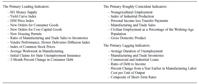
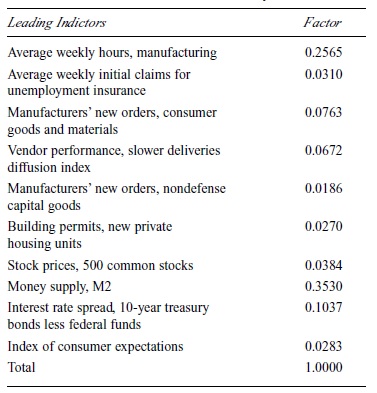
Table 2. U.S. Composite Leading Indexes: Components and Standardization Factors: February 2008

Economic research organizations use various schemes and models for generating a consensus interpretation for each group. For example, if the information used is limited to just the sign and magnitude of a change, the Conference Board produces diffusion indexes for all three groups. In addition, if the relative importance of the individual indicators is used, the Conference Board has composite indexes, such as composite leading economic indicators. AIER has similar indexes derived using different schemes. These factors are also used informally, usually by economic experts with extensive experience in economic forecasting, to produce a consensus interpretation for a group. Thus, given the high degree of subjectivity involved in this process, economists often arrive at different interpretations of the same information and produce different assessments of the state of the economy.

Another way to use these indicators to identify the position of an economy in a business cycle is to combine the information and interpretations of all three groups of indicators. If the changes in indicators of all three categories behave the same way, either positively or negatively, it is an indication that the economy is in a given state of the business cycle: expansion if the changes are positive and recession if the changes are negative. However, when the signs are different, they may point to a peak or trough of the cycle. In an expanding economy, negative changes in leading indicators, no change in coincidental indicators, and positive changes in lagging indicators are a sign of a possible peak in the economy. Similarly, in a declining economy, positive changes in the leading indicators, no change in the coincidental indicators, and negative changes in the lagging indicators are a sign of a trough in the economy. There are formal, econometric methods used for such analysis, which are briefly mentioned in the next section. However, it is the subjective interpretations of the information by the expert economists that are frequently used for decision making—a method that may result in even more conflicting interpretations!

Combining Information and Predicting a Turning Point

In the previous section, economic indicators were described. We noticed that some of these indicators can be grouped as lagging indicators, coincidental indicators, and leading indicators. We have also noted that the values of these indicators could be used in a group to describe the overall state of an economy at a given time.

In this section, we focus on combining information from these indicators and using them to predict the near future state of an economy in a business cycle. The idea is that, for example, if there are 10 leading indicators that all individually describe the behavior of the state of an economy in the near future, a composite, a combination, of them should have a superior performance over the performance of each individual one—superior in yielding more accurate predictions and signaling fewer false alarms. A false alarm would be an indicator that signals a recession when in fact one is not likely to occur.

The question then becomes how to combine the information provided by the indicators and how to evaluate the performance of a composite indicator in identifying the state of an economy on a business cycle. Modeling and nonmodeling approaches are used in response to these questions. Both approaches are briefly described in this section. A detailed treatment of these approaches is quite mathematical, requiring a high level of understanding of mathematical and econometric modeling—something that is well beyond the scope of this introductory research paper (Lahiri & Moore, 1991). For interested readers who have a good technical grasp of economic modeling, a rather comprehensive treatment of these topics is the excellent collection of work presented in Graham Elliott, Clive Granger, and Allan Timmermann (2006).

Modeling Overall Economic Performance

To model an economy’s overall performance, several measures are used to capture different areas of economic activity. For example, because employment and production are two very important aspects of an economy, measures and indicators of these aspects, such as unemployment rate and industrial production, are both used in the analysis.

Because each measure provides information about a particular aspect of the economy, for studying an economy’s overall behavior, a combination of these measures, a composite indicator, must be used.

GDP is the one indicator that is generally recognized as a good measure of the overall state of an economy. A disadvantage of GDP, however, is its low production frequency (quarterly as opposed to monthly). Other monthly indicators such as industrial production (IP), real personal income, and employment can, however, be used as proxies for GDP. These proxy indicators are not perfect, and their relative importance continually changes due to changes in the structure of an economy.

A more appropriate measure of the overall economic performance seems to be a composite measure of several indicators. The National Bureau of Economic Research (NBER) uses a combination of such measures as IP, employment, income, and sales in an informal, committee process for making decisions on business cycle dating. The Conference Board uses a formal, statistical method for combining the information of the individual indicators to produce lagging, coincidental, and leading composite indicators. There are also econometric-based models for formally combining information. These formal methods are briefly described next.

Statistical Modeling

The purpose of statistical modeling is to identify a set of indicators that collectively represents all important aspects of an economy; to measure the indicators’ statistical properties, such as their means, standard deviations, and correlation coefficients; and to combine this statistical information to produce composite indicators. The best-known such indicators are the Conference Board’s composite lagging indicator (CLgl), composite coincidental indicator (CCI), and composite leading indicator (CLI) (Conference Board, 2001). The CLI is the most used as a predictor of the near future state of the U.S. economy.

CLI is a linear weighted-average value of 10 leading indicators of the U.S. economy whose assigned weights are standardized values of their relative variability, with standard deviation of an indicator used as a measure of variability. The higher the variability of an individual indicator (high standard deviation), the lower weight assigned to it in the composite. These weights are standardized to a total of 100% for all 10 indexes.

CLI values are produced monthly starting at a base value of 100 at a given month and year and adjusted for the changes in CLI every month after. Thus, an increase in CLI value over its previous month is considered a positive growth in the economy (i.e., increase in real GDP value), and a decrease in CLI value is considered a negative growth (i.e., a contraction). This base month and year is updated every few years. The latest update started in April 2008 by setting the CLI value for January 2004 equal to 100.

CLI’s components and weights are regularly updated and revised to be current with the changing economy.

Weight distribution is updated annually, reflecting the addition of new information used in statistical measures. However, more fundamental revisions happen less frequently and are made only when there is good evidence indicating a change in relative predictability of the individual leading indicators. This usually reflects a possible structural change in the economy.

The last such modification happened in 1996 when the Conference Board recognized that financial and money indicators were more accurate in predicting the near future state of the U.S. economy than the real economy indicators. A decision was made to replace three of the real economy indicators with two new money indicators. A revised distribution of the weights assigned a much higher total relative weight of about 65% to the money indicators and a much lower total weight of 35% to the real economy indicators. As a result of this revision, two money indicators of interest rate spread and money supply received over 60% of the total CLI weight.

This revision was troublesome because these two money indicators are also monetary policy instruments that, to a large extent, are controlled and influenced by the Federal Reserve Bank policy decisions. The implication is that monetary activities were to a large extent dominating CLI. In other words, CLI was less influenced by the activities of the real economy. This problem became obvious in the 2001 recession when CLI did not provide good forecasting information about the near future state of the economy. The Conference Board has, subsequently, made a revision to the definition of the interest rate spread in 2005, resulting in a reduced relative weight being assigned to it in CLI.

Criticisms of the statistical modeling of a composite indicator focus on its lack of underlying support in economic theory and on its not tracking a specific target similar to the one used by econometric modeling. However, from a practical viewpoint of being able to predict the near future state of the economy, especially in predicting and dating peaks and troughs in business cycles, the CLI has been very informative and accurate. In addition, CLI information is easy to understand and communicate to nontechnical consumers and beneficiaries (i.e., business decision makers) of such information.

Econometric Modeling

Econometric modeling of composite indicators relies on cause-and-effect relationships supported by economic theory. Leading and coincidental indicators are modeled. Two approaches, factor-based modeling and Markov switching (MS) modeling, are used to model the composite coincidental indicator. For the development of the composite leading indicators, three approaches—vector autoregression (VAR)-based modeling, factor-based modeling, and MS-based modeling—are discussed next.

Econometric modeling of composite indicators is theoretical and complex, and requires a high degree of understanding of underlying technical issues. From the practical point of view of capturing and predicting the overall behavior of the economy, the performance of these indicators is, at best, as good as that of indicators developed using statistical modeling.

The rationale behind factor-based modeling is that there are a number of common forces behind the movements of coincidental indicators. An econometric model that incorporates these common factors is developed to estimate the coincidental indicators (Sargent & Sims, 1977; Stock & Watson, 1989). The rationale behind MS modeling is the same with the exception of relaxing the assumption of a fixed dynamic behavior of the economy in a business cycle. In other words, as the economy goes through expansion and recession phases in a business cycle, the model parameters are changing or switching according to a probabilistic behavior of the Markov process (Hamilton, 1989). Justification behind MS modeling is that economic factors behave and interact differently in recession and expansion phases of a business cycle.

The rationales described here for factor-based and MS-based construction of composite coincidental indicators are also valid for the construction of the composite leading indicators (CLI). Because the main purpose of producing the CLI is predicting the near future state of the economy, the information generated from these models can be used to produce the probability of a turning point in an economy and to devise a decision rule for signaling a downturn point and a recession.

VAR is a linear model for establishing a relationship between leading indicators and coincidental indicators and their lagged values. Once a model is established, in a similar way to the other composite leading indicators’ econometric models, its results can be used for business cycle predictions.

In addition to the approaches mentioned already, there are other mathematical approaches to developing leading indicators. One approach is incorporating a smooth transition to MS modeling. This approach assumes that the phases of the business cycle transition from one to another (i.e., expansion to recession) gradually rather than abruptly and suddenly. A second approach uses artificial neural networks to tap into a vast class of nonlinear models of the relationship between leading indicators and coincidental indicators. There is still another approach using binary variables in modeling expansion and recession phases of a business cycle and applying probit and logit methods for estimation and prediction. Massimiliano Marcellino (2006) is a good starting point for learning about modeling.

Evaluation

A model is evaluated for its performance using insample data and out-of-sample data. In either case, this evaluation can be formal or descriptive. The purpose of the in-sample evaluation is to check for the fitness of the model to the sample data. Selection of a formal evaluation is a function of the forecasting methodology applied. For example, in cause-and-effect modeling of a target variable, such as the coincidental composite indicator as a linear function of leading indicators, standard statistical and econometric evaluative methods can be used. Formal methods for out-of-sample evaluation range from mean squared error (MSE) and mean absolute error (MAE), used if the target variable is a continuous variable such as a leading indicator, to quadratic probability score (QPS) and log probability score (LPS), used for predicting a discrete indicator such as an upturn or downturn in an economy (Diebold & Rudebusch, 1989; Winkler, 1969). A comprehensive treatment of forecast evaluation can be found in Kenneth D. West (2006).

A shortcoming of formal evaluation methods is that they are based on the information of the data series for the entire period of study, and every data point is given the same amount of weight in the analysis. In reality, data points around the peaks and troughs of a business cycle are more important for evaluating a turning point, and special attention should be given to them.

Descriptive evaluations of the models, which can be used for both in-sample and out-of-sample periods, are usually most effective in identifying the peaks and troughs ofa business cycle. The goal is to measure how accurately and timely a model signals a turning point in an economy and to identify false alarms and missed signals. Descriptive evaluation methods are more informative in communicating the performance of a turning-point forecasting model.

A model that predicts a peak with a lead time is superior in its forecasting. Generally, the longer this lead time is, the better that model is. The number of consecutive downturn signals identified by a model is a measure of how persistent a model is in signaling a peak. The larger this value, the greater the likelihood that a peak will occur.

Forecasting and Economic Policy Making

Economic climate is extremely uncertain and volatile during a slowdown, downturn, and peak period. The state of the economy, and the information about it, can change drastically in a very short period of time. A forecast is made based on the best information available at a given time, and an economic policy formulated using this forecast may become nonaccurate and ineffective to counterproductive, respectively, once the information has changed. This may create challenges for economists dealing with all stages of measuring economic indicators, of forecasting state of the economy, and of making policy recommendations. The contemporary state of the U.S. economy (2007-2009) has provided a clear example of this situation described as follows:

2007 to 2008 Second Quarter: Two major factors dominated the economic climate in this period.

1. Factor 1 is a substantial and continuing decline of the housing prices throughout the country after 5 years of major growth year after year. This has created two distinct problems for the economy with direct and, possibly, major effects on many economic activities. The first problem is a decline in the number of new housing construction permits and in the construction of the new houses. The second problem, also known as the subprime mortgage rate crises, is the substantial readjustment increases of the variable mortgage rates as a result of the rise in the interest rates to the effect that a large number of these mortgages are not affordable to the homeowners. Nonaffordability of mortgage payments coupled with decline in housing prices have forced many banks to foreclose on people’s houses. Because most of the mortgage contracts are securitized and sold in market to financial institutions throughout the world, it was unclear at this point how a large number of mortgage defaults could have an impact on these institutions in the coming months and years.
2. Factor 2 is the rapid increases in the commodity prices, from oil to soy beans, in the last few years, due to increase in demand from the emerging developing countries, which had put a substantial upward pressure on the prices of many goods and services from grocery products to plane tickets.

Confronting inflation in the economy is a primary policy objective of the Federal Reserve System for bringing stability in the economy. In formulating a monetary policy at that time, the Federal Reserve had to deal with the conflicting consequences of these two factors on the economy. On one side, it had to raise interest rates in order to confront inflation in the economy. On another side, it had to ease the supply of money in order to confront the economic slowdown consequences of a decline in housing construction and of instabilities in the financial institutions. The balancing policy actions of the Federal Reserve System in dealing with these problems were critical in preventing a peak in the U.S. economy in 2007 to 2008.

By summer 2008, all indications were that, of the two major factors impacting economic stability, the threat of the subprime mortgage rates effects was being diminished and inflation was going to be the main concern going forward. Therefore, what happened in the economy in late 2007 to early 2008 seemed most likely to be a slowdown, not a recession. The recommended policy action was an anti-inflationary policy of raising interest rates and reducing money supply.

2008 to 2009: Moving on to fall 2008, a sudden change occurred in the status of these two economic factors. It turned out that the impacts of the subprime mortgage rates on the financial institutions were so deep that they basically paralyzed the entire industry, requiring substantial governmental interventions, at the U.S. and global levels, to prevent it from collapsing. This brought slowdowns, downturns, and recessions to the countries around the world. In fact, in December 2008, NBER officially declared a recession for the United States starting December 2007. Given such a state of the economy globally, inflation did not turn out to be a concern, mainly due to a collapse in the commodity prices. The recommended policy was an expansionary policy of cutting interest rates and providing stimulus fiscal help.

Economic Indicators and Forecasting in the Twenty-First Century

An economy, as a dynamic system, is continuously changing to incorporate technological innovations in the production processes and to satisfy the needs of an ever-evolving society. In the last 30 years, an outburst of technological innovations in the computer and in communication has moved the economy to be more global. This can clearly be seen in the formation of the global corporations in all industries, especially in financial, and in the outsourcing of production and services in the manufacturing and labor sectors. The global slowdown and recession of 2007 to 2009 has taught us that there is a strong interaction among the economic activities of all countries around the world. We are seeing that new economic powers are emerging in the developing countries, challenging the already well-established powers of the United States, the European Union, and Japan. These new powers are strong in both producing and consuming goods and services. At such a global setting, the economy of a country is very much dependent on global economic activities. This dependency needs to be incorporated in measuring economic parameters of a country, such as output, prices, employment, and so on. In addition, new parameters need to be identified and measured for the global economy. Further studies along these areas are expected in the years to come.

On the technical aspect of forecasting, one area that still needs substantial contribution is in applied forecast evaluation. Defining success in an organization and evaluating the performance of a forecast in that context is in critical need of development. For example, in predicting the overall state of the economy in the near future, is a forecast of a downturn that did not happen, due to the policy makers’ effective and timely actions, a failure or a success? It can easily be argued that that forecast was a false alarm, thus, a failure. However, that predication has generated new information to alert the policy maker to act, thus it is a success. Developing objective evaluation methodologies of the performance of a forecast in the context of an organization’s overall objective can be very helpful. For people interested in performing research on the technical areas of forecasting, a starting point is the excellent survey of Elliott et al. (2006).

Bibliography:

1. Burns, A. F., & Mitchell, W. C. (1946). Measuring business cycles (NBER Studies in Business Cycles No. 2). New York: National Bureau of Economic Research.
2. Conference Board. (2001). Business cycle indicators handbook. Available from https://www.conference-board.org/pdf_free/economics/bci/BCI-Handbook.pdf
3. Diebold, F. X., & Rudebusch, G. D. (1989). Scoring the leading indicators. Journal of Business, 62(3), 369-391.
4. Elliott, G., Granger, C., & Timmermann, A. (Eds.). (2006). Handbook of economic forecasting (Vol. 1). Amsterdam: Elsevier North-Holland.
5. Hamilton, J. D. (1989). A new approach to the economic analysis of nonstationary time series and the business cycle. Econometrica, 57, 357-384.
6. Lahiri, K., & Moore, G. H. (1991). Leading economic indicators: New approaches and forecasting records. Cambridge, UK: Cambridge University Press.
7. Marcellino, M. (2006). Leading indicators. In G. Elliott, C. Granger, & A. Timmermann (Eds.), Handbook of economic forecasting (Vol. 1, pp. 879-960). Amsterdam: Elsevier North-Holland.
8. Sargent, T. J., & Sims, C. A. (1977). Business cycle modeling without pretending to have too much a priori economic theory. In C. Sims & C. W. Granger (Eds.), New methods in business cycle research (pp. 45-109). Minneapolis, MN: Federal Reserve Bank of Minneapolis.
9. Stock, J. H., & Watson, M. W. (1989). New indexes of coincident and leading economic indicators. In O. Blanchard & S. Fischer (Eds.), NBER macroeconomics annual (pp. 351-394). Cambridge: MIT Press.
10. West, K. D. (2006). Forecast evaluation. In G. Elliott, C. Granger, & A. Timmermann (Eds.), Handbook of economic forecasting (Vol. 1,pp. 100-134). Amsterdam: Elsevier North-Holland.
11. Winkler, R. L. (1969). Scoring rules and the evaluation of probability assessors. Journal of the American Statistical Association, 64, 1073-1078.