Experimental Economics Research Paper

This research paper provides an introduction to laboratory methodology in economics, an overview of a small selection of results indicating examples of what has been learned from this research with an emphasis on how such learning can be linked with data and theory outside of traditional economics. Also the use of the laboratory as a test-bed for economic systems design is briefly discussed. Where possible, references will be to citations and discussion in Davis and Holt (1993), Friedman and Sunder (1994), Kagel and Roth (1995), and Smith (1991).

1. What Is An Economics Experiment?

Every microeconomy (laboratory or field) can be represented by three elements. (Smith 1991, pp. 255–

71). The first is the environment, specifying agent characteristics that motivate action. In neoclassical economics this included agent endowments, preferences, and technology (costs). In laboratory experiments monetary rewards are most often used to induce a specific value cost environment and to motivate decision. The institution defines the language (messages) of agent communication, the rules (property rights) governing the exchange of information, allowable actions (moves), and how messages actions lead to valued outcomes. Laboratory experiments use instructions and decision forms (often computer controlled) to define the institution. Finally, there is the observed behavior of agents subjects given the environment and institution. Here are three examples of laboratory microeconomies

1.1 Trust Game (Fig. 1)

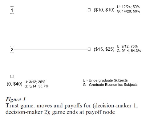
1.1.1 Environment. The alternative payoffs are shown in the outcome parentheses for (DM1, DM2), where DMi is decision-maker i =1, 2. Thus, at the bottom of the decision tree, conditional on reaching node 2, if DM2 moves down, the payoffs are (DM1, DM2) = ($0, $40).

1.1.2 Institution. Subjects, for example, in groups of at least 12, are randomly and anonymously paired, and randomly assigned the roles (1 or 2). DM1 moves first, choosing right, in which case the game ends with payoffs ($10, $10), or down. If down, DM2 chooses right yielding ($15, $25) or down ($0, $40). Each player sees the moves in sequence of the other. No communication is permitted (except the moves); neither DM knows with whom he she is paired. Variations on this institution might include players not seeing each other’s moves; being able to communicate or play might be repeated with the same unknown person. The experimental protocol—rules and procedures—define the institution in an experiment.

1.1.3 Behavior. Shown next to each payoff outcome is the (proportion; percentage) of all subjects ending at the indicated payoffs for each of two subject population samples:

(a) Undergraduates (U) with various majors; the typical subject.

(b) Graduate (G) students in economics, from across the US and Europe in their third or fourth year of study, attending a workshop in experimental economics.

For a discussion of bargaining experiments and further references see Davis and Holt (1993, pp. 241–75), Friedman and Sunder (1994, pp. 56–60), Kagel and Roth (1995, pp. 253–348), and McCabe et al. (1996).

1.2 Auction Experiments

1.2.1 Environment. Subjects, for example, in groups of four, are each assigned one value, Vtε [0, $10], chosen independently with replacement, where each value is equally likely to be drawn for each i in each auction period, t=1, 2, …, T, where T is unknown to the bidders. Vi is the maximum willingness-to-pay of i for one unit of the abstract good in period t, since if i wins the auction he/she earns Vi – (price paid)i. At each t one unit is offered for sale to the four competing bidders at zero supply price.

1.2.2 Institution (Sealed High-Bid Auction). At t each i submits a b_i^d≥0, the high bidder wins and pays a price equal to the amount bid. Hence, if i =1 is the high bidder, his her earnings are Vt -bt .

1.2.3 Behavior. Subjects tend to submit bids that are approximately proportional to their assigned value, i.e., bi =αiVi, where αi is i’s estimated bid coefficient based on all observations (bt, Vt). If all bidders are risk neutral, the Bayes–Nash theory predicts αi=N-1/N=n/4 with N =4, for all i. If agents are risk averse, their bid coefficient is αi>3/4 . This is because, so it is argued from the theory, that they are willing to accept less profit, Vt bt, to increase the chances of being the high bidder. Almost all bidders (over 90%) in high-bid experimental auctions bid as if they are risk averse. See Davis and Holt (1993, pp. 275– 308), Friedman and Sunder (1994, pp. 107–9), Kagel and Roth (1995, pp. 501–85), and Smith (1991, pp. 509–661) for references and discussion of experimental auctions.

1.3 Double Auction Stationary Supply And Demand Experiment

1.3.1 Environment. M buyers are assigned one or more positive values in period 1. Each buyer earns V_i -P_i for each unit with value V_i that is purchased at price P_i; each of N sellers earns P_j -C_j on each unit sold at price P_j, where C_j >0 is one of the costs assigned to seller j in period 1. The same values and costs might be assigned in period 2 and all subsequent periods, defining a stationary replicating economic environment.

An example is provided in the experiment of Fig. 2 in which there are six buyers, each with a capacity to buy up to three units. Buyer 1 has a three-unit demand schedule. His three maximum willingness-to-pay limit prices are at $20, $13.50, and $13.20 as indicated by the three units designated by B1 in Fig. 1. If B1 buys a first unit, he earns $20 minus the purchase price; a second unit earns $13.50 minus its purchase price and so on. Other buyers have limit price demand schedules as shown. When all limit prices are pooled and sorted from highest to lowest this defines the market demand schedule of prices and corresponding maximum purchase quantities.

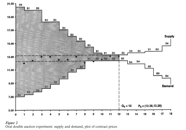
Similarly, sellers are assigned minimum willingness-to-accept limit selling prices. For example, seller S4 can sell up to three units at unit costs $7.00, $13.50, and $14.50, respectively. When all seller limit prices are sorted from lowest to highest we get the market supply schedule, shown in Fig. 2.

Each buyer and seller only knows his or her private local supply or demand schedule. As Hayek would say, information is dispersed; each agent knows his or her own particular circumstances of time and place which we summarize in the form of the indicated limit values and costs in Fig. 2 (Hayek 1945, cited in Smith 1991, p. 234). Supply is to order in the environment shown in Fig. 2 so that there is no carryover of units not sold and therefore not supplied. In a multiple period competitive market experiment the supply and demand schedules so defined become flows per period. Note that any P_E in the interval ($12.30, $13.20) is a competitive equilibrium that clears the market of 12 units. The theoretical gains from exchange are represented by the shaded area of Fig. 1. Keep in mind that no subject in the experiment knows this, and none sees before them a chart like Fig. 1. This information is unnecessary.

1.3.2 Institution. We also need an institution that defines the language of the market and its operating rules. In the example of Fig. 2 we use the bid-ask double auction rules common in financial and commodity markets. Any buyer (seller) can announce a bid (ask) price to buy (sell). Agents are recognized one at a time with bids and asks written into a spread sheet in sequence on an overhead. Once a bid (ask) is established a new bid (ask) must be higher (lower). Hence, the bid-ask spread is required to narrow. At any time any buyer (seller) can accept the standing ask (bid) to form a contract. For example, seller S1 might sell her first unit to buyer B6 at price $12. The seller earns a profit of $12-$8.20 =$3.80 and the buyer a profit of $20-$12=$8. This process continues for, say, 5 minutes or until no new contracts are forthcoming. The first market period ends, and the market opens for a new trading period. There are many software programs allowing these rules to govern trading via computer terminals.

1.3.3 Behavior. With M, N=3 or more, the sequence of contract prices tends to be volatile at first, then converge, within a few trading periods, to near the competitive equilibrium price and quantity that equalizes the quantities demanded and supplied (Smith 1991, Davis and Holt 1993, Chap. 3). But in Fig. 2 the subjects (Department of Energy administrators) were especially good traders, and prices stayed very close to the P_E interval during the first period. The contract prices for each trade are plotted as dots in the order of their occurrence: the first at $12, then $12.40, etc., the 11th and 12th at $13. Al- though 12 units traded the market was 97 percent efficient (not shown), just short of 100 percent. Efficiency is the percentage of the shaded area that is collected as gains from exchange (profit) in any period. What was the source of inefficiency? Buyer B2 bought his third unit (the 13th market demand unit in order; value $12.30) from one of the lower cost sellers at the price $12.20 on the 9th contract as plotted. If a demand unit below P_E trades, this displaces one of the higher value demand units that must trade if the market is to be 100 percent efficient. Full efficiency is achieved only if the highest 12 demand units are satisfied by the 12 lowest cost supply units, with all other units not trading. Otherwise, further gains from exchange can be realized. In this case buyer B2 could resell his unit to the higher value buyer he displaced, yielding a profit for each. In the experiment shown, no provision was made for such retrading.

Double auction markets are studied in Davis and Holt (1993, pp. 125–72), Friedman and Sunder (1994, pp. 18–20), Kagel and Roth (1995, pp. 368–72), and Smith (1991, Parts I and II).

2. What Have We Learned From Experiments?

2.1 Personal Vs. Impersonal Exchange: Reconciling Cooperative And Noncooperative Behavior

The results reported in the trust game of example 1.1 above contrast with those in the single unit auction, example 1.2, and the double auction example 1.3, posing an anomaly. Why do half of the subjects choose cooperative strategies in anonymous two-person games, such as Fig. 1, while, universally, subjects behave noncooperatively in anonymous interaction first price auctions and in double auctions (Fig. 2)?

To see the problem, consider the predictions of theory in the game of Fig. 1. Agents are assumed to be self-interested maximizers who choose dominant strategies, and who assume that any paired counterpart does the same. Thus, if player 2 gets a chance to move, she receives $40 by moving down, $25 by moving right. Player 1, expecting player 2 to choose her dominant strategy ($40), will not play down. Thus, the noncooperative equilibrium (NE) of the game is for player 1 to move right yielding ($10, $10).

An alternative theory, prominent in social and evolutionary psychology, postulates that there are reciprocity types in the population who follow reputational lifestyles in social interactions, normally cooperating with other like persons. They also reciprocate when others offer cooperation to them. All social exchange among friends, associates, and ingroup members involves trading favors, services, and gifts, with deep roots across all cultures including hunter-gathers. The sense of indebtedness for a favor is expressed in the common phrase, ‘I owe you one.’ For such types a move down by DM1, followed by a move right by DM2, constitutes an exchange. Each incurs a potential opportunity loss (Player 1, $0-10=-$10; player 2, $25-40=-$15) for a potential gain of 50 percent for player 1 and 150 percent for player 2 relative to NE. The exchange requires trust by DM1 and trustworthiness by DM2. Experimentalists originally used anonymous matching protocols to control for such pair-bonding. Therefore one of the important discoveries was that this protocol controls very poorly for such phenomena.

Even graduate students in economics with knowledge and training in game theory do not predominantly apply the NE model in Fig. 1. One interpretation is that the reciprocity model is so strong and innate that it overcomes the effect of such training.

Thus, in an important sense, reciprocity behavior in Fig. 1, and noncooperative behavior in experimental markets, such as Fig. 2, are not anomalous: both achieve efficient–maximum gain—outcomes. In the former, an example of personal exchange, coordination on efficient outcomes, requires shared attention, intentionality detection, and ‘mindreading’ (Baron-Cohen 1995) by reciprocity types; in impersonal exchange in markets, coordination through a pricing institution achieves efficient outcomes which are not part of the intention of agents who, noncooperatively, seek only their own gain. One cannot speak of an identifiable ‘other mind’ to be read. In Smith (1998) it is argued that reciprocity, in the extended family and the tribal societies of our hunter-gatherer ancestors, would have laid the exchange foundation for specialization and wealth creation millennia before the emergence of long-distance exchange based on barter, and, ultimately, something that would be called ‘money.’ (Also see North 1990 on personal vs. impersonal exchange and the emergence of long-distance trade.)

2.2 Institutions Matter

The rules governing social and economic interactions matter because they affect the state of agent information, perception, and incentives, which in turn affect decisions. Because information on value (cost) is dispersed among agents the frequency and content of the messages exchanged are important elements in equilibrium price discovery. This is demonstrated at the elementary level in single-object auctions. In the English ‘open outcry’ auction (E), if each bidder knows only his own value, then after the initial bid each bidder has an incentive to raise the standing last bid if it is below the bidder’s valuation for the item, but never to raise his own standing bid. Consequently, the bids increase until the highest value bidder eventually raises the standing bid until it is equal to or just above the second highest value bidder, and he or she is awarded the item at the price equal to the last bid. The award is thus efficient, and experiments tend to confirm the high efficiency and price predictions of this theory. The E auction, however, is vulnerable to collusion, since a subset of friends/associates may refrain (reciprocally) from raising each other’s bids even in the absence of formal agreement. In the absence of collusion, no one is motivated to invest in information about the values or bidding strategies of others (which would be socially wasteful) because bids and withdrawals are public information, although the identity of those taking the actions may not be public.

In the first price sealed bid auction (F), the high bidder also wins and pays his bid price, but each bidder bids once, blind to the bids of others. In F, bids are also related to value, but also to what a bidder may know, guess or believe about the valuations of others, and, theoretically, to his own attitude toward risk. Information on the bids or values of others is informative, and bidders are motivated to invest in acquiring such information. Knowing the highest bid of your competitors enables you to win with a slightly higher bid, and leave no money on the table.

A variation of the F auction is the second price sealed bid auction (S), in which the highest bidder wins but pays the seller a price equal to the second highest bid submitted. Whoever wins is put in the position of being a price-taker, i.e. the amount of the winning bid determines the probability of winning but has no effect on the profit from bidding. Therefore it is a dominant strategy to bid your value, thus maximizing expected profit; if all do this, the high value bidder wins at a price equal to the second high value. This logical characteristic of S auctions is not immediately trans-parent to unsophisticated bidders, although many learn over time to bid their value without necessarily being able to articulate why.

In the Dutch auction (D) the price starts high and descends until the first bidder stops the clock (in Dutch flower auctions) or yells ‘mine’ (in Spanish fish auctions): the auction is over with the first (public) bid. It is a theorem that the D and F auctions are isomorphic: it is rational to stop the clock at the price you would bid in the F auction. Behaviorally, in D auction experiments, on average, subjects tend to let the clock run below the level at which they would bid in an F auction (Cox et al. 1983 in Smith 1991, pp. 580–94). Note that collusion is difficult in D auctions because no one knows what might be the highest of your competitor’s bids because it is never observed.

Theoretically, under the Vickrey assumptions (e.g., risk-neutral bidders), the above auctions all yield the same efficient allocations and expected price. With risk averse bidders, the E and S auctions are still equivalent and efficient, the D and F auctions are equivalent, but not efficient, and yield higher average prices than E and S. This is an example in which the environment interacts with the institution: with risk aversion bidders’ behavior in D and F diverges from that in E and S. Behaviorally, in lab experiments, E and S auctions are roughly equivalent, and highly efficient, with comparable average prices. The D and F auctions are not equivalent; F prices are higher, and have higher efficiency: in both D and F bidders bid as if they were predominantly risk averse. (For surveys see Davis and Holt 1993, Friedman and Sunder 1994, Kagel and Roth 1995, and Smith 1991.)

2.3 Stock Market Bubbles Are Common In The Laboratory

Finance theory teaches that the value of an equity share is determined by its fundamental value: the expected discounted value of its future yield (or dividends). Consider a simple environment for testing this hypothesis: N =(9 or 12) subjects are each given an endowment of cash and shares; at the end of each of 15 trading periods a dividend is drawn from the four alternatives (0, $0.08, $0.28, $0.60), each with a probability of one-quarter of yielding an expected dividend of $0.24 per period. Hence, during the first period each individual has a right to 15 draws from this dividend distribution, so that fundamental value is 15×($0.24)=$3.60; during the second period the right is to 14 draws, and value is 14×($0.24)=$3.36, and so on. This information and these calculations are displayed to all subjects to guard against any misunderstanding (see Smith et al. 1988 in Smith 1991, pp. 339–71).

In Fig. 3 the white bars plot the declining theoretical (dividend) value, from $3.60 in period 1 to $0.24 in period 15. A typical experiment using inexperienced undergraduate subjects is indicated by the black bars that plot the average double auction contract price by period: average prices start below fundamental value, rise over time to above this value, then crash a few periods before the end, approximating the fundamental value by periods 14–15. Perhaps 100 such experiments have been reported in the literature documenting this bubble/crash behavior for inexperienced subjects, and the fact that only when a group is brought back for a third session do prices finally approximate the fundamental value. The interpretation is that common information is not sufficient to yield common fundamental value expectations; it is not enough because each person still has uncertainty about the behavior of others. It is through a common experiential process that subjects resolve this behavioral uncertainty and approach common expectations.

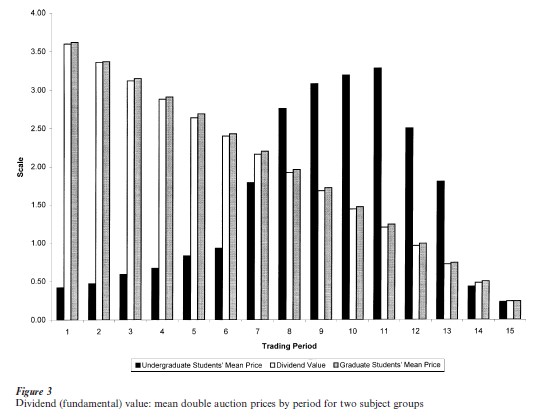
But suppose that advanced graduate students participate in this experiment. A subset of 22 subjects from the sample who participated in the trust game, whose results are depicted in Fig. 1, also participated in an asset trading experiment, yielding mean prices represented by the gray bars in Fig. 3: mean prices deviate no more than five cents from fundamental value. Hence, in this market game, advanced students in economics are rational, and expect others in their group to be rational. Common information and knowledge of others’ types is sufficient to yield common rational expectations. For a comprehensive survey of asset trading, see Sunder, pp. 445–500 in Kagel and Roth 1995).

2.4 Rewards And Decision Costs Matter

The examples of environments in Sect. 1 all use salient cash rewards for the subjects; i.e., payment is directly related to earnings from decisions. Subject moves in Fig. 1 have substantial payoff consequences, while in market experiments buyers are motivated to buy at low, and sellers to sell at high, prices (see Davis and Holt 1993, pp. 24–26). There are many studies over the past 40 years showing that reward level matters. There are also cases showing that increased rewards do not improve performance (Smith and Walker 1993). Even when the central tendencies of the data support theoretical predictions, increased reward can cause the variance of the observations to decline as the data clusters more closely around theoretical predictions. Where the data do not support the predictions of a theory, increased payoffs may cause the data to move closer to those predictions, although statistically the predictive hypothesis is still rejected (see Smith and Walker 1993 for a survey). Psychologists sometimes interpret this to mean that rewards have ‘little or no effect.’ (Certainly the ‘effect’ may not rescue the theory.) Alternatively, when theory fails, a common critique from economists is that the payoffs, in particular the payoff deviations from the predictions, were inadequate (Kagel and Roth 1995, pp. 66–7). This is the methodological problem of flat maxima: even with substantial rewards, as in an auction experiment, bidding above or below the optimum may reduce payoff by only a small amount.

Notice that the findings that the variance, or distance, of the observations from the predictions declines with rewards, and the interpretations, that the rewards have little effect, or change only slightly with deviations from optimality, are all extra theoretical issues. The theory predicts the unique optimum, with zero deviation/variance, however gently rounded is the payoff function. Thus, the ex post hoc claim that the opportunity cost of deviating from optimality is ‘too low’ is implicitly a claim that other resource costs, pertinent to a decision, are not included in the theory. If the rewards are adequate, then such costs would be overcome and the decision would be closer to the theory. Economic theories of optimal behavior ignore decision costs—the costs of thinking, calculating, attention, monitoring, deciding, etc. Stakes are not a formal part of the theory, and payoff adequacy tends to surface only as an afterthought when a theory performs poorly in tests.

This problem illuminates the key methodological issue in any experiment: an experiment is a joint test of a theoretical hypothesis and everything you choose to do (procedures, relative and level of payoffs, information provided, etc.) to implement the test. This is why, whenever a theory fails replicable testing, it is most important to re-evaluate both the theory and the testing apparatus (laboratory or field) as a system. Otherwise, one can always interpret the test as rejecting the auxiliary hypotheses used in the test, and not the theory: every time you double the stakes, the test either succeeds or fails; if it fails one concludes that the stakes were inadequate; if it succeeds one concludes that the theory is correct. This defines a process in which the theory cannot be falsified. Yet in traditional economics all basic theory development tends to abstract from the issues that arise in implementing a test. In the above example, the pattern of observed deviations from predictions begs for some formal extension of theory that takes rewards into account. (For a discussion of methodology in experimental economics, see Smith 1991, pp. 783–801.)

We briefly outline a simple such extension based on a model of subjects’ decision cost (Smith and Szidarovszky 1999). Consider an interactive game among N decision-makers, with payoffs π_i(y₁,…, y_N) given the decision choices, y_i, for each i. Let y_i =x* define a Nash equilibrium in the standard paradigm of unbounded, costless, rationality. Now let y_i=x*_t-ε_t(z_t) where ε_t(z_t) is agent i’s error deviation from equilibrium, depending on the cognitive effort, z_i≥0. More effort is productive, implying that ε_i(z_i) is decreasing in z_i. But reduced error increases payoff. From the perspective of the decision-maker, reward net of cognitive cost, C_i(z_i), is π_i(x*_i-ε_i(z_i),…, x*_i– ε_i(z_i),…, x*_N– ε_N(z_N))-C_i(z_i). This defines a modified equilibrium in which effort cost is balanced against its value in reducing error. For optimal z_i=0, we get the testable implication that increasing payoffs reduces average error, and the variance of error.

This model also explains what can go wrong when increasing the stakes has an insignificant effect on performance, as is often found across the range of experiments: the decision task has very high effort cost and/or effort has low productivity in reducing error. Then, decision costs may dominate the effect of larger rewards. Also it can be seen why subject experience might be as, or more, important than reward level. Experience allows decisions to become routine, with reduced attentional effort. Learning initially to play a Bach sonata may be arduous even for a skilled pianist, who performs with little effort and without conscious thought once it is mastered. Thus, rewards may sometimes be more effective for inexperienced than experienced subjects (see Jamal and Sunder 1991, cited in Friedman and Sunder 1994, p. 220).

3. How Can Experiments Be Applied In The Field?

Beginning over 30 years ago experimental methods have been employed to study a wide variety of phenomena with direct application outside the laboratory (Smith 1991, pp. 511–14). The worldwide privatization deregulation movement over this period has created a great demand for ‘test bedding,’ the use of the laboratory to test the performance properties of new kinds of markets and to train participants in the field. (For some discussion and further references see Davis and Holt 1993, pp. 296–304, Kagel and Roth 1995, pp. 119–21, Friedman and Sunder 1994, pp. 32–7, Smith 1991, pp. 662–702, Rassenti and Smith 1998).

Thus, laboratory experiments have been used to inform the design of pollution credit trading, natural gas production, delivery and transmission, spot markets in electricity, and recently the auction of rights to the spectrum.

These constitute examples of smart computer assisted markets, in which optimization algorithms are applied to the decentralized messages submitted by agents. Such systems combine the information advantages of decentralized private property rights and ownership with the coordination advantages of central processing. The control center is not a decision- making unit; it merely applies coordinating, allocation, and pricing algorithms to the messages of decentralized owners. The center itself can be organized as a rule-governed joint venture of the private users in which entry is required to be open for new users who invest in the expansion of capacity. The first smart computer assisted market was a combinatorial auction that selected combinations of elemental items, valuable only in packages, that were responsive to the package bids of independent agents. (see Rassenti 1981, cited in Smith 1991, p. 677, Rassenti, Smith and Bulfin 1982, cited in Smith 1991, pp. 662–77). Fig. 4 compares the efficiency of a combinatorial auction, in the panels on the right, with an independent auction of the components of the multiple discrete units that comprise the packages.

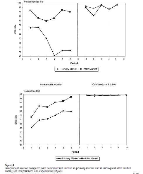
Each auction period consists of two markets, a primary market represented by either the independent (uniform price sealed bid) auction or the combinatorial auction of packages, followed by an open book after market allowing traders to post bids to buy or sell for elements or combinations of elements. The after market enables bidders to obtain valued elements missing from packages they attempted to piece together in the independent auction, or packages they failed to obtain in the combinatorial auction. Six elementary resources were available, each in fixed supply. Six bidders each had induced values for four, five, or six packages of the six elements. For example, a bidder had a value of 887 for the package (1, 0, 1, 0, 1, 0) consisting of one unit each of resources A, C, and E. If all three elements are obtained, the bidder receives 887. If any element is missing the value is zero. The upper panel results are for two groups of inexperienced subjects, while the lower panel uses experienced subjects. With inexperienced subjects, comparing the results at the end of each primary market for the independent and combinatorial auctions, efficiency in the latter was larger than that in the former in every period. The same holds for the after market comparisons, except the improvement from primary to after market is much greater in the independent auction. This is because almost all of the high efficiencies in the combinatorial auction were achieved in the primary auction, which, for experienced subjects, is 98–99 percent efficient.

Bibliography:

1. Baron-Cohen S 1995 Mindblindness. MIT Press, Cambridge, MA
2. Davis D D, Holt C A 1993 Experimental Economics. Princeton University Press, Princeton, NJ
3. Friedman D, Sunder S 1994 Experimental Methods. Cambridge University Press, Cambridge, UK
4. Kagel J H, Roth A E 1995 Handbook of Experimental Economics. Princeton University Press, Princeton, NJ
5. McCabe K, Rassenti S, Smith V 1996 Game theory and reciprocity in some extensive form experimental games. Proceedings of the National Academy of Sciences of the USA 93: 13421–8
6. North D C 1990 Institutions, Institutional Change and Economic Performance. Cambridge University Press, Cambridge, UK
7. Rassenti S, Smith V 1998 Deregulating electric power: market design issues and experiments. In: Chao H, Hunting H G (eds.) Designing Competitive Electricity Markets. Kluwer, Boston
8. Smith V 1991 Papers in Experimental Economics. Cambridge University Press, Cambridge, UK
9. Smith V L 1998 The two faces of Adam Smith. Southern Economic Journal 65: 2–19
10. Smith V, Szidarovszky F 1999 Monetary rewards and decision cost in strategic intentions. Unpublished manuscript
11. Smith V, Walker J M 1993 Monetary rewards and decision cost in experimental economics. Economic Inquiry 35: 245–61