Aggregate Demand and Aggregate Supply Research Paper

People often assume that textbooks present settled theory. It might therefore be a surprise to some that economists do not universally accept the AD/AS model. It has, in fact, been the subject of a heated debate. Critics of the model charge that it is an unsuccessful attempt to combine Keynesian and neoclassical ideas about the macroeconomy. Detractors also contend that it sacrifices accuracy for the sake of easy pedagogy.

The purpose of this research paper is to examine the model and a few of the charges leveled against it. The first part of the research paper presents the model as it usually appears in textbooks. The presentation includes applications and a discussion of policy in the context of the model. Following that is a discussion of some of the main criticisms. We discover that the critics may have a point.

Theory

The Aggregate Demand Curve

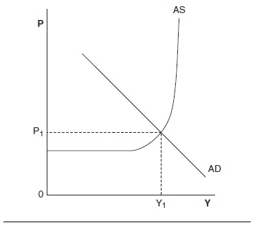
The aggregate demand curve is drawn as a negatively sloped curve in price level/real gross domestic product (GDP) space (see Figure 1). It shows how real aggregate spending is influenced by changes in the price level. Aggregate spending is the sum of consumption, desired investment, government purchases of goods and services, and net exports, symbolized as C + I + G + NX. At the principles level, there are usually three explanations given for why real aggregate spending varies inversely with the price level: the wealth effect, the interest rate effect, and the foreign trade effect.

The wealth effect is also known as the real balance or Pigou effect. All else equal, as the price level rises, people who hold money discover that they can buy less with their money. In other words, they experience a decrease in the real value of their wealth held as money. As a direct result, they will buy fewer goods and services as the price level rises.

Figure 1   The Basic AD/AS Model SOURCE: Adapted from Reynolds (1988, p. 221).

The interest rate effect is sometimes called the Keynes effect. To understand it, one must first understand the theory of liquidity preference, which is the idea that in the short run, interest rates are determined by the supply of and demand for money. In the money market, the nominal supply of money is determined by the central bank. The nominal demand for money depends on real income, the price level, and the nominal interest rate. All else equal, as real income rises, people will buy more goods and services. To do so, they will need more money. As the price level rises, people will need more money to carry out the same volume of real transactions. Money demand is negatively related to the interest rate because the rate of interest is the opportunity cost of holding money. All else equal, as the interest rate rises, people will reduce the amount of money they want to hold.

The equilibrium short-run interest rate is the rate that causes the quantity of money demanded to equal the quantity of money supplied. If the interest rate is too high, there will be a surplus of money in the sense that people will want to hold less money than they do. To reduce money holdings, people will buy bonds and deposit money in interest-bearing accounts. The result will be a fall in the rate of interest. If the interest rate is too low, the opposite will occur. People will want to hold more money than they have. To obtain it, they will sell bonds and withdraw money from interest-bearing accounts, and that will drive the interest rate up.

The liquidity preference theory is in contrast to how interest rates are determined in the long run. In the long run, interest rates are determined in the market for loanable funds—that is, by national saving, domestic investment, and net capital outflow (also known as net foreign investment). According to the doctrine of long-run money neutrality, the supply of money cannot influence the real interest rate in the long run.

So what is the interest rate effect and how does it affect the slope of the aggregate demand curve? There are two different approaches presented in textbooks that are logically equivalent. In one approach, an increase in the price level increases the nominal demand for money. For a given money supply, the increase in money demand drives up the rate of interest. A higher interest rate reduces consumption and desired investment spending. In other words, a higher price level drives up the rate of interest and thereby reduces the real quantity of output demanded.

The other approach conceives of the money market in real terms. By dividing the nominal money supply and nominal money demand by the price level, one gets real money supply and real money demand. Holding the nominal money supply constant, as the price level rises, the real money supply falls. The fall in the real money supply creates a shortage of money at the prevailing interest rate, so the interest rate rises. As with the other approach, the higher interest rate reduces consumption and desired investment and therefore reduces the real quantity of goods and services demanded.

There are two versions of the foreign trade effect. The first approach is direct: As the domestic price level rises, exports fall and imports rise as buyers substitute foreign goods for the more expensive domestic goods. The second approach, often called the exchange rate effect, follows from the interest rate effect. As the price level rises, the interest rate rises. A higher interest rate makes domestic bonds more attractive. As a result, domestic residents will want to buy fewer foreign bonds, and foreign residents will want to buy more domestic bonds. In the market for foreign exchange, that translates into a decrease in the supply of the domestic currency and an increase in the demand for domestic currency. That will cause the value of the currency (the exchange rate) to rise. A rise in the exchange rate means that domestic goods become more expensive relative to foreign goods. Exports will fall and imports will rise. In other words, the increase in the price level will reduce net exports, and so the real quantity of output demanded falls.

Be aware that the aggregate demand curve is not just the summation of all market demand curves, and the reasons for their negative slopes differ. For a market demand curve, a change in price is considered holding all other prices constant. It therefore represents a change in relative price. A market demand curve is negatively sloped because a relative price change creates income and substitution effects. A higher price causes people to substitute away from the good, and it reduces their real income. For a normal good, lower real income reduces the quantity of the good purchased. For the aggregate demand curve, a price change represents an absolute change in the overall price level. There can be no income effect for the macroeconomy as a whole because when the overall price level rises, both the prices people pay and the prices people receive increase. For every buyer there is a seller, so one person’s higher expense is another person’s higher income. To the extent that people buy more foreign goods and fewer domestic goods as the domestic price level rises, there can be a type of macroeconomic substitution effect. But as we shall see, this effect is likely to be small.

At the intermediate level, the interest rate effect is emphasized, though the other two are sometimes mentioned. In intermediate courses, the aggregate demand curve is typically derived from an IS/LM model. The interest rate effect is clearly illustrated in the IS/LM framework, as a higher price level shifts the LM curve left (upward). The result is a higher interest rate and lower real GDP in equilibrium. To the extent that the higher interest rate drives up the exchange rate, the IS curve will shift left (downward) as net exports fall. The wealth effect of a higher price level reduces consumption and so also shifts the IS curve to the left (downward). In all three cases, a higher price level is associated with lower equilibrium real GDP.

There is an alternative derivation of the aggregate demand curve based on the quantity equation, MV = PY, where M is the money supply, V is the income velocity of money, P is the price level, and Y is real GDP. MV is total spending on final goods and services. For a given value of MV P and Y must be inversely related. In this formulation, the aggregate demand curve is a rectangular hyperbola. This version of the aggregate demand curve is less popular and is used primarily to show how changes in the money supply affect aggregate demand (Mishkin, 2007). It is less useful for showing how individual components of spending affect aggregate demand. That is because one would have to explain how a change in investment, for example, affects velocity.

The Aggregate Supply Curve

There are two distinct textbook approaches to aggregate supply. In the simpler version, the aggregate supply curve is horizontal at the current price level for all values of output below full employment, and vertical at full employment. The idea is that as long as there is unemployment, increases in aggregate demand will increase output, not prices. Once the economy reaches full employment, further increases in demand can only drive up prices. A slightly more sophisticated version of this approach has a positively sloped region as the economy nears full employment (see Figure 1). The idea is that some industries will reach full employment before others, so as demand rises, some industries will respond by increasing output, while other industries will be unable to produce more and so will raise prices.

The second approach is more sophisticated and leans heavily on the research about the Phillips curve done by Nobel laureates Edmund Phelps (1967) and Milton Friedman (1968). Phelps and Friedman argued that there was a short-run trade-off between inflation and unemployment, but that the trade-off vanished in the long run. In other words, a higher inflation rate may allow the economy to move above its full-employment level of output temporarily, but not permanently.

The aggregate supply version of the Phillips curve analysis posits a long-run aggregate supply curve that is vertical at the full-employment level of output (see Figure 2). This corresponds to the economy’s “natural” rate of unemployment that allows for only frictional and structural unemployment, but no cyclical unemployment. It is vertical because, in the long run, real GDP is determined by real forces such as the availability of resources and technology, not by the price level. Over time, the long-run aggregate supply curve will shift right as technology improves and as the economy acquires more capital and labor. Its position is also affected by tax rates and other things that affect the incentives to supply capital and labor, create businesses, and develop new technology.

Deviations from full employment can occur when the actual price level deviates from the expected price level. There is no consensus as to why this is the case, but three different explanations are commonly presented (Mankiw, 2007).

Figure 2 The Enhanced AD/AS Model SOURCE: Adapted from Mankiw (2007, p. 762).

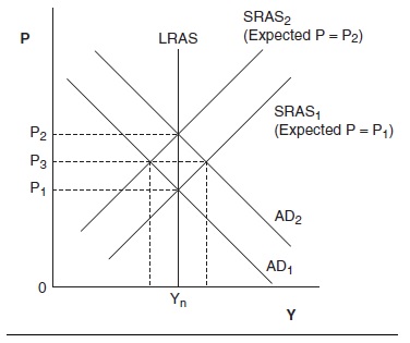
One explanation, called the sticky-wage model, is based on the idea that wages are not perfectly flexible and may be fixed in the short run. Wages are set based on some expected price level, so if prices turn out to be higher than expected, real wages will be lower than expected. In response, firms will hire more workers and increase output. In other words, the aggregate supply curve will have a positive slope in the short run. The effect will not persist, however, because nominal wages will eventually adjust to reflect the higher level of prices. When price expectations are adjusted upward, workers will demand higher wages. Employment will then return to its long-run value. In terms of the model, the short-run aggregate supply curve will shift left (see Figure 2).

Another explanation for the short-run aggregate supply curve’s positive slope begins with the observation that many prices are sticky. That means that some firms change their prices only periodically. The prices of raw commodities like grain and metal may fluctuate daily, or even hourly, but prices of finished goods behave differently. B. Bhaskara Rao (1993) found that over 85% of U.S. transactions on final goods and services take place in “sluggish price” markets. That means that sticky prices are quite common. One reason is markup pricing. Price setters often set price by adding a markup over marginal cost. Fluctuations in demand are met with changes in output, not price. A second reason is fear of competitors. Firms do not want to be the first to raise price for fear of losing customers to competitors. A third reason is menu costs: It is expensive to frequently reprint catalogs and price lists. Moreover, when firms do change their prices, they do not all do so at once. That means that as the overall price level rises, the relative price of the output produced by firms with sticky prices falls. As a result, they experience higher than normal sales. In response, the firms increase output. The result is that a rising price level is associated with rising real GDP. Once again, however, the effect is only temporary. When the firms change their prices, they will adjust them upward in line with the overall price level. The result is that their sales will decline and output will fall. That implies that the short-run aggregate supply curve shifts to the left (see Figure 2).

A third explanation assumes that some firms are temporarily fooled. When the price of their output rises due to an increase in the overall price level, these firms misperceive it as an increase in the relative price of their output. In response, they increase production. As in the previous two cases, the increase in real GDP is only temporary. Firms will eventually correct their perceptions and recognize that the relative price of their output has not increased. When that happens, they will reduce production. The short-run aggregate supply curve will shift left (see Figure 2).

All three of these explanations can be represented in a single equation,

Y = Yn + a(P-Pe)

where Y is actual real GDP, Yn is the long-run or “natural” rate of real GDP, a is a positive constant, P is the actual price level, and Pe is the expected price level. The equation shows that when the actual price level deviates from the price level that was expected, real GDP will deviate from its natural rate. In the long run, when expectations adjust to reality, the price level will equal the expected price level, so real GDP will equal its natural rate.

The Adjustment to Equilibrium

As in so many other economic models, equilibrium is where the lines cross. Suppose, for example, that in Figure 2, AD2 is the relevant aggregate demand curve and SRAS2 is the relevant short-run aggregate supply curve. The economy is in both short-run and long-run equilibrium with the price level at P2 and real GDP at its “natural” level, Yn. Then suppose that aggregate demand falls to ADr At P2, the amount of real GDP people want to buy is less than the amount firms want to sell. In the short-run, the excess supply will cause the price level to fall to P3 and real GDP to fall below Yn. Because the actual price level (P3) is below the expected price level (P2), real GDP is below its long-run value. Over time, price expectations will fall, and the short-run aggregate supply curve will shift to the right. This effect will be reinforced by the cyclical unemployment that exists when real GDP falls below Yn. Unemployment puts downward pressure on wages, and that will reduce firms’ costs. Eventually, the economy will return to Yn with a price level equal to Pj. At that point, the short-run aggregate supply curve will be at SRASJ in Figure 2.

Applications and Empirical Evidence

The primary application of the model is to predict and explain short-run fluctuations in real GDP around its longrun trend. It is intended to explain how recessions and booms occur, and why the economy tends to return to its natural rate of real GDP. According to the model, deviations from the economy’s long-run trend are the result of shocks to either demand or supply.

Demand Shocks

For a given price level, a change in any of the components of aggregate demand will shift the aggregate demand curve. Recall that aggregate demand is the sum of consumption and desired investment, government purchases of goods and services, and net exports. A change in any of these can shift the aggregate demand curve. If any of them fall, aggregate demand will shift to the left. As detailed at the end of the previous section, that will cause a temporary decline in real GDP, otherwise known as a recession. If any of the components rise, aggregate demand will shift right. For example, in Figure 2, begin with ADJ and SRASJ. At Pj and Yn, the economy is in short-run and long-run equilibrium. If aggregate demand rises to AD2, the short-run result is an increase in the price level to P3 and an increase in real GDP above Yn. The economy is in a boom period. Eventually, price expectations will be revised upward, and the short-run aggregate supply curve will shift left to SRAS2. When that happens, the boom is over and the economy returns to its long-run trend.

The key point is that fluctuations in aggregate demand cause fluctuations in real GDP. The components of aggregate demand are each influenced by a large number of variables. It is therefore not surprising that aggregate demand fluctuates. The model shows how fluctuations in demand are translated into fluctuations in real GDP.

Of all of the components of aggregate demand, desired investment spending is the most volatile. As John Maynard Keynes (1936/1964) emphasized, investment is extremely sensitive to the state of expectations. That is because investors face known present costs and uncertain future returns. The decision to build a factory is an act of faith. The investor can never be certain what future demand for the factory’s output will be. A recession may suppress demand and lower price. Technological change may make it obsolete. There is no way to precisely calculate the return on the factory, and Keynes argued that one typically does not even know enough to establish probabilities. It is no surprise that waves of optimism or pessimism among investors can lead to significant fluctuations in investment, aggregate demand, and real GDP.

Consumption spending is also affected by the state of expectations, though to a lesser degree. That is primarily because spending on necessities such as food, shelter, and transportation cannot be avoided. But consumption spending on some goods, such as furniture and entertainment, can be postponed. An old sofa can be made to last longer. If consumers fear a recession that might put their jobs in jeopardy, they will try to save more and consume less. If they are optimistic and believe that the economy will boom, they may expect higher income in the future. That could lead them to save less (or borrow more) and consume more now.

Export demand depends to a significant degree on the health of our trading partners’ economies. If one or more of them go into a recession, their demand for our exports will fall. That, in turn, will reduce our aggregate demand. Other things equal, the result would be to create a recession here too.

While the model correctly predicts that a decline in aggregate demand will reduce real GDP, it also predicts that the overall price level will fall. One weakness of the model becomes apparent when one realizes that the overall price level in the United States has not fallen over the course of a year since 1955. One would be hard-pressed to argue that there have not been any negative demand shocks over that period. Defenders of the model argue that there are other forces in the economy that keep the price level rising even in the face of falling aggregate demand. They contend that falling aggregate demand puts downward pressure on prices—that is, will slow the rate of growth of prices. That may well be true, but that is not what the model says. As some economists have argued, the model is much better at explaining output movements than price movements.

Supply Shocks

Broadly speaking, there are two types of supply shocks: input-price shocks and technology/resource shocks. Input-price shocks lead to sudden changes in the expected price level and therefore shift the short-run aggregate supply curve. Technology/resource shocks affect the economy’s production function and shift both the long-run and the short-run aggregate supply curves.

Input-Price Shocks

The aggregate demand and aggregate supply model became popular primarily because of the oil price shock that hit the West in the mid-1970s. The model was able to correctly predict the consequences of the shock. The 1973 Arab-Israeli war led Arab oil-exporting countries to embargo the West. The price of oil more than doubled in a short period of time. The price of oil is important because it contributes to the cost of producing and distributing almost everything. Inputs must be shipped to factories and output must be shipped to stores. Workers must travel to work. When the price of oil increased suddenly, people understood that costs, and therefore prices, would soon increase too. In other words, the expected price level increased, so the short-run aggregate supply curve shifted to the left.

In terms of Figure 2, begin with AD1 and SRAS1, with the economy in long-run equilibrium at P1 and Yn. The higher expected price level shifted the short-run aggregate supply curve to SRAS2. In the short run, the price level rises to P3, and real GDP falls below Yn. The combination of falling output and rising prices is often called stagflation. The U.S. economy saw an increase in the unemployment rate from 4.9% in May of 1973 to 9.0% in May of 1975. Over the same period, the price level as measured by the Consumer Price Index increased 21.15%. A second oil-price shock hit the United States in the late 1970s, when the price of oil again more than doubled. The results were similar. The unemployment rate increased from 6.0% in May of 1978 to 7.5% in May of 1980, and the price level rose 26.69% over the same period.

In the mid-1980s, the price of oil moved sharply in the other direction. From 1982 to 1986, the price of crude oil fell more than 50%. The drop in the price of oil reduced the expected price level and shifted the short-run aggregate supply curve to the right. In terms of Figure 2, begin with AD2 and SRAS2, with the economy in long-run equilibrium at P2 and Yn. The fall in the expected price level shifts the short-run aggregate supply curve to SRAS1. The model predicts that the price level will fall to P3 and real GDP will rise above its natural rate. As the model predicts, the U.S. unemployment rate fell from 9.4% in May of 1982 to 7.2% in May of 1986. The price level rose 13.65% over the same period, contrary to the model’s predictions. An explanation is that aggregate demand increased over the period, which would tend to drive up the price level.

Technology/Resource Shocks

The aggregate demand and aggregate supply model is designed to explain business cycles, but it is worth briefly mentioning a few long-run effects. Improvements in technology raise the productivity of a nation’s resources and thereby increase the natural rate of GDP. As a result, both the long-run and short-run aggregate supply curves shift to the right. The acquisition of more resources through immigration, natural population growth, and capital accumulation will have the same effect on the two curves. This is another way of saying that in a growing economy, the natural rate of GDP will rise over time.

Policy Implications

The AD/AS model as usually presented suggests that the economy will recover from adverse shocks on its own. Yet some economists argue that the process may take a long time. That is because the price level may be slow to adjust, especially in the downward direction. In other words, sticky prices and sticky wages may significantly delay the restoration of full employment. The model offers guidance to those who believe that policy can speed the process along.

Policy Responses to Demand Shocks

If aggregate demand falls, real GDP will fall and unemployment will rise. Either fiscal policy or monetary policy (or both) can be used to increase aggregate demand. Fiscal policy uses the government’s power to spend and tax. To boost aggregate demand, the government can increase its own spending or it can cut taxes so as to stimulate private spending. The net effect on aggregate demand depends on the relative magnitude of two conflicting forces. One is the multiplier effect. An increase in spending raises the income of those who receive the new spending. They, in turn, will spend some of their new income, which will raise the income of somebody else. In this fashion, the initial increase in spending can induce additional spending elsewhere in the economy. The net result is that total spending in the economy can rise by a multiple of the initial increase.

The second effect is called crowding out. The increases in income set in motion by the multiplier effect will raise the demand for money. That will cause the interest rate to rise, which will reduce investment, consumption, and net exports. In this fashion, the initial fiscal policy action can “crowd out” other forms of spending. The crowding out will reduce the amount by which aggregate demand rises. The net effect on aggregate demand depends on the relative strength of the multiplier and crowding out effects.

Monetary policy can also be used to raise aggregate demand. If the central bank increases the money supply, the rate of interest will fall. That, in turn, will tend to raise investment, consumption, and net exports. Keynes argued in his General Theory (1936/1964) that monetary policy may be ineffective in a severe recession or depression because even very low interest rates may not raise spending sufficiently if investors and consumers have pessimistic expectations about the future.

Policy Responses to Supply Shocks

Policy makers face a dilemma when confronted with an adverse supply shock. Suppose a price shock shifts the short-run aggregate supply curve to the left, which raises prices and reduces output and employment. If policy makers raise aggregate demand in order to restore full employment, the price level will rise even more. If policy makers lower aggregate demand in order to stabilize prices, output and employment will fall even farther. Any policy that changes aggregate demand will make either inflation or unemployment worse.

The only policy that might work to reduce both inflation and unemployment would be one that acts directly on the short-run aggregate supply curve. The options open to policy makers are limited. One possibility is to reduce business and payroll taxes in order to reduce business costs. To the extent that such a move would counteract the increase in costs caused by the price shock, the expected price level might be reduced. That would shift the short-run aggregate supply curve back to the right.

Future Directions

The appeal of the AD/AS model is obvious. Its superficial similarity to the familiar market demand and supply model makes it easy to teach. That, together with the power of habits of thought and inertia, suggests that the model has a bright future. But as was mentioned in the introduction, the model has its critics.

The Slope of the Aggregate Demand Curve

Consider the three reasons given for the negative slope of the aggregate demand curve. The wealth effect is much discussed, but the estimates are that it is trivially small. Nobel laureate James Tobin (1993) estimated that the wealth effect is so weak that a 10% drop in the price level would increase spending by only 0.06% of GNP. In other words, major changes in the price level would not have much of an effect on aggregate spending. As Bruce Greenwald and Nobel laureate Joseph Stiglitz (1993) argue, the excessive attention given to the wealth effect “hardly speaks well for the profession” (p. 36).

Another problem with the wealth effect is that it is selective about what types of wealth are affected by a price-level change. Specifically, it ignores the effect of a change in the price level on the real value of debt. A price-level decrease, for example, will increase the real value of debt. And while it is true that the real gains to creditors equal the real losses of debtors, the effect on spending is not neutral. This is for two reasons. The first is that, by definition, the propensity to spend is higher for debtors than for creditors. That means that the price-level decrease will reduce the economy’s overall propensity to spend. The second reason is that a falling price level makes it harder to repay debt. One can reasonably expect, and history has amply demonstrated, that a decrease in the price level will increase the proportion of bad loans and the number of bankruptcies. Taken together, the implication is that a fall in the price level is likely to reduce the real value of spending, not increase it as the aggregate demand curve claims.

The foreign trade effect also has problems. The version of it that argues that a higher price level will make domestic goods more expensive and so reduce net exports is strictly true only if the exchange rate is fixed. If the exchange rate is flexible, then one would expect the rising domestic price level to reduce the value of the currency. The price increase and the currency depreciation should roughly cancel each other out, with minimal effect on net exports. The other version argues that the higher interest rate associated with a higher price level will drive up the exchange rate and so reduce net exports. Yet once again, the higher price level will itself reduce the value of the currency. The overall effect on net exports will be small.

According to Tobin (1993), the interest rate effect was first discussed by Keynes (1936/1964). Yet Keynes himself did not put much faith in it. The main reason is that changes in the price level that trigger the interest rate effect are likely to alter expectations. This illustrates a central problem for the model: In discussions of short-run aggregate supply, expectations have a central role. Yet in discussions of the aggregate demand curve, expectations are completely ignored. Consumers and investors are implicitly assumed to never change their price expectations.

Consider the reasonable possibility that an increase in the price level will cause people to expect even higher prices in the future. A normal reaction might be to buy more now to avoid paying even higher prices later. If that happened, the aggregate demand curve could have a positive slope. Alternatively, if the aggregate demand curve is drawn holding price expectations constant (as it is), then it would shift to the right when the price level increased.

The more general point is that it is not at all clear that a higher price level will reduce the quantity of goods and services people buy. At best, the aggregate demand curve is extremely steep, almost vertical. If that is the case, then why bother to put the price level on the vertical axis at all? As was suggested earlier, the model is much better at predicting changes in real GDP than it is at predicting changes in the price level. The prominent role of the price level in the model is no doubt an attempt to blend neoclassical economics (which views price adjustments as the primary equilibrating force) with Keynesian economics (which views output adjustments as the primary equilibrating force). The result is not always satisfactory.

Incompatibility of the Aggregate Demand and Aggregate Supply Curves

The aggregate demand curve is in no sense a behavioral relationship like a market demand curve. The aggregate demand curve is a set of equilibrium points. This is seen clearly when the aggregate demand curve is derived from the IS/LM model, as it usually is in intermediate macroeconomics classes. The intersection of the IS and LM curves shows the equilibrium rate of real GDP where both the goods market and the money market are in equilibrium. As the price level changes, the LM curve shifts. By repeatedly changing the price level, one can generate an aggregate demand curve that shows the relationship between the price level and the rate of real GDP where the goods market and money market are both in equilibrium.

Implicit in this story is the assumption that production rises along with demand to keep the goods market in equilibrium (Barro, 1994; Nevile & Rao, 1996). As the price level falls and the LM curve shifts right (downward), the rate of interest falls and spending rises. This is the familiar interest rate effect. Output is assumed to be forthcoming to match the increase in spending. It is a manifestation of Hansen’s law that demand creates its own supply. To put the matter differently, the derivation of the aggregate demand curve implies that firms can always sell everything they care to produce at whatever the price level happens to be.

The logical problem should now be apparent. The aggregate supply curve presents a much different relationship between the price level and the level of output that firms produce. Worse yet, the AD/AS model argues that if the price level is above its equilibrium value, then there will be an excess supply of goods. How can that be when the aggregate demand curve is derived with the assumption that the goods market is in equilibrium?

One cannot argue that the aggregate demand curve is a notional demand curve akin to a market demand curve, where the relationship between price and quantity demanded is hypothetical. Instead, the aggregate demand curve shows us what the market clearing level of output is at various price levels. And if the market is clearing, there cannot be an excess supply. This inconsistency is the primary reason that prominent macroeconomist Robert Barro (1994) said that the model is “unsatisfactory and should be abandoned as a teaching tool” (p. 1).

David Colander (1997) argues that the aggregate demand curve should be called the aggregate equilibrium demand curve so that its nature is apparent to students and professors alike. He goes so far as to say that the aggregate demand curve was deliberately named incorrectly in order to mislead students into thinking that macroeconomics was nothing more than “big micro.”

Colander also argues that an aggregate supply curve may not exist for the same reason that a supply curve does not exist in an imperfectly competitive market. In such markets, output decisions cannot be separated from demand. A price-setting firm must choose price and output at the same time and cannot do so without reference to demand. Colander argues that most firms charge a markup over cost, and the amount they produce is based on expected demand. It is therefore impossible to create a supply function independent of the demand function.

The fundamental point is that in a Keynesian short-run world, output adjusts to clear markets. In a neoclassical long-run world, prices adjust to clear markets. The AD/AS model is an attempt to have it both ways. In it, price-level changes work to equate the quantity of real GDP demanded and supplied even in the short run. To do so, there must be separate supply and demand functions. But if Keynes and Colander are correct, one cannot separate production decisions from demand.

Conclusion

In a famous article, Friedman (1953) argued that the real test of a model is how well it predicts. As noted previously, the AD/AS model became popular primarily because it correctly predicted the effects of the price shocks of the 1970s. It also does a pretty good job of predicting how shocks to the economy affect real GDP. But the model predicts that a decrease in aggregate demand or an increase in aggregate supply will reduce the price level, and that has not happened in the United States for over 50 years. Certainly aggregate demand has fallen and aggregate supply has increased in the last half century. Defenders of the model argue that what the model is really saying is that such events put downward pressure on the price level, so that the rate of inflation will decrease. Yet that begs the question as to why the model has the price level on the vertical axis instead of the inflation rate.

Models with the inflation rate on the vertical axis exist and occasionally appear in textbooks (Jones, 2008; Taylor &Weerapana, 2009). These models typically derive the aggregate demand curve from a monetary policy rule (Taylor’s rule) that describes how the central bank reacts to changes in the inflation rate. As the inflation rate rises, the central bank increases the nominal interest rate by more than the rise in the inflation rate. The effect is to increase the real interest rate, which reduces the real volume of spending. The approach avoids the problems with the aggregate demand curve discussed previously. John B. Taylor and Akila Weerapana’s model has no aggregate supply curve. Instead, the microfoundations of price setting are discussed for the purpose of emphasizing how inflation is self-perpetuating in the short run. Charles Jones uses a variant of the Phillips curve as an aggregate supply curve. Critics of these models complain that they lean too heavily on a policy rule that may not always exist. Yet all models ultimately depend on specific institutions (such as property rights) and habits of thought. To look for a macroeconomic model devoid of an institutional foundation is to look for a chimera.

The fundamental problem is that the macroeconomy is a dynamic, complex thing. Static models cannot capture its nuances. A model simple enough to teach to undergraduates is bound to have flaws; in teaching, there is always a trade-off between accuracy and accessibility. The real question then becomes the extent to which the model convinces students of things that are not true.

Thomas Kuhn (1962/1996) famously observed that displacing well-entrenched theories is never easy. For one thing, the need for an alternative is not always clear to most scientists, and some actively suppress any heresies. It is safer to go along with the conventional wisdom. For a new approach to succeed, it must be clearly and demonstrably superior. If the AD/AS model is ever to be replaced, its critics must develop superior alternatives.

Bibliography:

1. Barrens, I. (1997). What went wrong with IS-LM/AS-AD—and why? Eastern Economic Journal, 23, 89-99.
2. Barro, R. J. (1994). The aggregate-supply/aggregate-demand model. Eastern Economic Journal, 20, 1-6.
3. Brownlee, O. H. (1950). The theory of employment and stabilization policy. Journal of Political Economy, 58, 412-424.
4. Colander, D. (1995). The stories we tell: A reconsideration of the AS/AD analysis. Journal of Economic Perspectives, 9,169-188.
5. Colander, D. (1997). Truth in labeling, AS/AD analysis, and pedagogy. Eastern Economic Journal, 23, 477-482.
6. Dutt, A. K. (1997). On the alleged inconsistency in aggregate supply/aggregate demand analysis. Eastern Economic Journal, 23, 469-476.
7. Dutt, A. K. (2002). Aggregate demand-aggregate supply analysis: A history. History of Political Economy, 34, 322-363.
8. Dutt, A. K., & Skott, P. (1996). Keynesian theory and the aggregate supply/aggregate-demand framework: A defense. Eastern Economic Journal, 22, 313-331.
9. Fields, T. W., & Hart, W. R. (2003). Bridging the gap between interest rate and price level approaches in the AD-AS model: The role of the loanable funds market. Eastern Economic Journal, 29, 377-390.
10. Friedman, M. (1953). The methodology of positive economics. In Essays in positive economics (pp. 3-43). Chicago: University of Chicago Press.
11. M. (1968). The role of monetary policy. American Economic Review, 58, 1-17.
12. Greenwald, B., & Stiglitz, J. (1993). New and old Keynesians. Journal of Economic Perspectives, 7, 23-44.
13. Hansen, R. B., McCormick, K., & Rives, J. M. (1985). The aggregate demand curve and its proper interpretation. Journal of Economic Education, 16, 287-296.
14. Hansen, R. B., McCormick, K., & Rives, J. M. (1987). The aggregate demand curve: A reply. Journal of Economic Education, 18, 47-50.
15. Jones, C. I. (2008). Macroeconomics. New York: W. W. Norton.
16. Keynes, J. M. (1964). The general theory of employment, interest and money. New York: Harcourt, Brace & World. (Original work published 1936)
17. Kuhn, T. S. (1996). The structure of scientific revolutions. Chicago: University of Chicago Press. (Original work published 1962)
18. Mankiw, N. G. (2007). Principles of economics (4th ed.). Mason, OH: Thomson-Southwestern.
19. McCormick, K., & Rives, J. M. (2002). Aggregate demand in principles textbooks. In B. B. Rao (Ed.), Aggregate demand and supply: A critique of orthodox macroeconomic modelling (pp. 11-23). London: Macmillan.
20. Mishkin, F. S. (2007). The economics of money, banking, and financial markets (8th ed.). New York: Pearson-Addison Wesley.
21. Nevile, J. W., & Rao, B. B. (1996). The use and abuse of aggregate demand and supply functions. The Manchester School, 64, 189-207.
22. Palley, T. (1997). Keynesian theory and AS/AD analysis: Further observations. Eastern Economic Journal, 23, 459-468.
23. Phelps, E. S. (1967). Phillips curves, expectations of inflation and optimal unemployment over time. Economica, 34, 254-281.
24. Rabin, A. A., & Birch, D. (1982). A clarification of the IS curve and the aggregate demand curve. Journal of Macroeconomics, 4, 233-238.
25. Rao, B. B. (1993). The nature of transactions in the U.S. aggregate goods market. Economics Letters, 41, 385-390.
26. Rao, B. B. (Ed.). (1998). Aggregate demand and supply: A critique of orthodox macroeconomic modelling. London: Macmillan.
27. Rao, B. B. (2007). The nature of the ADAS model based on the ISLM model. Cambridge Journal of Economics, 31, 4 1 3-422.
28. Reynolds, L. G. (1988). Economics (6th ed.). Homewood, IL: Irwin.
29. Saltz, I., Cantrell, P., & Horton, J. (2002). Does the aggregate demand curve suffer from the fallacy of composition? The American Economist, 46, 61-65.
30. Taylor, J. B., & Weerapana, A. (2009). Economics (6th ed.). New York: Houghton Mifflin.
31. Tobin, J. (1993). Price flexibility and output stability: An old Keynesian view. Journal of Economic Perspectives, 7, 45-65.
32. Truet, L. J., & Truet, D. B. (1998). The aggregate demand/supply model: A premature requiem? The American Economist, 42, 71-75.