Demand For Labor Research Paper

1. Static Theory

We can imagine an employer using technology, de-scribed by a production function, that links output Y to inputs such as labor, capital, materials, etc., all represented by L and a vector of other inputs X:

If we assume that the employer minimizes the cost of production, the demand for each input is determined by its own price (in the case of labor, the wage, w), other inputs’ prices, p_x, the product’s price, p, and the scale of the enterprise Y:

Throughout this research paper I subsume in w all costs of employment, including wages, nonwage monetary benefits paid to workers, and also nonmoney benefits. In studying the demand for inputs we typically set the product price equal to 1 , so that the input prices are adjusted for inflation. This labor-demand function then focuses on changes in employers’ labor inputs in response to changes in the wage rate (the own-price effect), prices of other inputs (cross-price effects), and total output (the scale effect). All of these responses are determined solely by the underlying technology summarized in the production function. In the end the demand for labor is a technological relationship, but one that is generated by cost-minimizing and often profit-maximizing behavior. Its derivation from under-lying economic motivations is similar to that of the consumer’s choice of goods and services.

A major focus since Marshall (1920) has been on the own-wage elasticity of labor demand—the percentage change in labor demanded in response to a 1 percent increase in the wage rate. Marshall offered four ‘ laws ’ describing the determinants of this elasticity. It is higher: (a) the more readily substitutable other inputs are for labor; (b) the easier it is for customers to switch away from the product when its price rises after an increase in labor cost; (c) the greater share that labor cost represents in the enterprise’s total cost; and (d) the more readily the supply of other inputs adjusts when a higher wage leads employers to attempt to switch away from labor and toward other inputs.

Measuring the wage elasticity of labor demand and the underlying technology that generates it has been the central empirical focus of the study of labor demand. The measurements answer the crucial question: if the cost of labor is raised, do employers cut the amount of labor they use, and by how much? The representation of technology that we use to infer the magnitude of this elasticity has become increasingly general over the years. The Cobb–Douglas function (Cobb and Douglas 1928) imposed the requirement that the own-wage elasticity equals (1–s) at each constant output level, where s is the share of labor in total cost. The Constant Elasticity of Substitution function (Arrow et al. 1961) allowed this elasticity to assume any constant value, but it required the cross-price elasticities of labor with respect to each other input to stand in the same ratio as the other inputs’ shares in costs. When we attempt to infer this elasticity today we either estimate it directly from labor-demand functions like Eqn. (2) or use generalized representations of technology, such second-order approximations as the translog function (see, e.g., Berndt and Christensen 1974). These approaches allow estimates of the own-wage and cross-price elasticities to take on any value indicated by available data on input quantities, their prices, and the scale of production.

The discussion thus far treats labor as if it were homogeneous, which is obviously wrong. One could expand Eqn. (1) to include labor disaggregated by any set of criteria of interest, for example, sex, race ethnicity, age, educational attainment, occupation, immigrant status, and others. In each of these cases Eqn. (2) expands into a system of equations, one for each group of workers, each containing the wage rates of each type of worker, other input prices, and scale Y. These expanded representations of technology allow researchers to examine how employers substitute among workers of different types. They generate estimates of cross-wage elasticities that indicate how the demand for one type of worker changes when the wage costs of others rise or when the prices of nonlabor inputs, particularly the cost of capital services, change. These may be positive, indicating that the two types of workers are p-substitutes, or negative, indicating that they are p-complements.

Equations (1) and (2) and the expanded versions that include several types of workers assume technology is unchanging. The existence of technical progress means that the demand for workers of different types may change even without changes in wage costs. Technical progress may, as seems to have been true in industrialized countries in the 1980s and 1990s, enhance the productivity of skilled relative to less-skilled workers and thus increase the relative demand for skill. With a limited supply of skilled workers this in turn raises their relative pay, partly choking off employers’ desires to employ more of them. The rate and nature of technical progress mean that the underlying technological parameters that determine own- and cross-wage elasticities are changing, so that the parameters themselves are not constant over time.

2. Inferring The Structure Of Labor Demand

Moving from the theory to inferring the sizes of the responses requires ensuring that we measure employers’ reactions rather than other behavior, particularly changes in the supply of labor. The issue is one of identification—inferring from simultaneous changes in such outcomes as wages and employment (either of all labor, or of particular groups of workers) which ones reflect employers’ responses. Consider Fig. 1, which shows two data points, A and B, describing combinations of wage rates and labor employed in a market observed at two different times, or in two different labor markets. Empirical economists might connect these two points, assume that they are traced out by changes in the supply of labor from S0 to S1, and infer that they lie along the demand curve for labor D. The percentage change in L relative to the percentage change in w between these points could then be used to measure the own-wage elasticity along this demand curve.

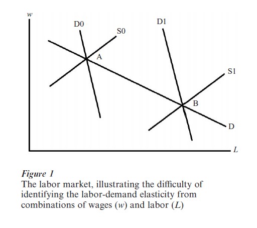
Making this inference might be wrong and mis-leading. Points A and B could have been generated by a shift in supply from S0 to S1 that was simultaneous with a shift in demand from D0 to D1. Labor demand might have shifted because product demand increased, because technology became more labor-using, or because the price of some p-complementary input to labor fell or that of some p-substitute rose. In that case the true demand elasticity (along D0 or D1) is smaller than the estimate one would obtain by ignoring the possibility that demand shifted. One must adjust for those factors that we believe shift demand ( px and Y in Eqn. (2)). Most importantly, one needs to find an exogenous source of variation in supply, so that we can be sure that the variations we observe in the combinations (w, L) are generated by shifts that are beyond employers’ control. After substantial concern until the 1960s about properly identifying labor- demand responses, it is only since the early 1990s that research on labor demand has refocused researchers’ attention on identifying changes in (w, L) combinations as reflecting movements along a demand curve.

3. Estimates Of Wage Elasticities

3.1 Sizes Of Responses

An immense body of empirical research has been devoted to measuring the own-wage elasticity of demand for homogeneous labor. Using data on employment, wages, and scale (output) of entire countries, major industries or small industries examined over time, or on individual employers at a point in time, researchers have attempted to pin down this central parameter in the theory of labor demand. Others have used similar data for other research purposes, with estimates of this parameter being a by-product of their investigations. Estimates have been produced for most industrialized countries and for many developing countries.

The central conclusion of the empirical literature on the demand for labor validates the principle of substitution. At a given scale of output, a rise in labor costs leads employers to substitute away from labor and toward other inputs whose cost has not risen. This is true in nearly all the over 100 studies summarized by Hamermesh (1993, Chap. 3) that were unconcerned about problems of identification. It is also true in the newer literature that pays special attention to ensuring that the slope of the demand curve is identified (e.g., Angrist 1996). With the many different sets of data and methods, the estimates of elasticity vary widely. Nonetheless, the bulk of estimates cluster in the range -0.15 to -0.75, with a ‘ best-guess ’ meta-analytic estimate being -0.30. At a given level of output, a rise in labor cost of 10 percent will eventually reduce employment by 3 percent as employers substitute toward technologies that use less of the now more-expensive labor and more of the now relatively cheaper other productive inputs.

The constant-output own-wage elasticity tells us the degree of substitution between labor and other inputs. That knowledge is useful, for example, for inferring how much extra employment is generated at a given level of output when employment is subsidized, or how much might be lost when payroll tax rates are raised. In order to infer the full effect on employment of labor taxes or subsidies, or of changes in other input prices, in an economy with some available labor (one that is not at full employment) we also need to add the scale effect of changes in labor costs. The evidence suggests that the scale effect is fairly substantial, probably larger than the substitution effect, so that the total elasticity of labor demand for the average employer may be as large as 1.0. Interestingly, this estimate, based on a very large body of empirical studies, is exactly what is implied by the simplest representation of technology, the Cobb–Douglas production function.

When Eqn. (2) is expanded into a system of demand equations describing several types of labor, our ability to draw fairly tight inferences about the sizes of the own-and cross-wage elasticities is diminished by the sheer number of possible disaggregations. The current literature says nothing definite about the absolute sizes of particular own-and cross-wage elasticities, and making progress on this front is high on the agenda for research in the next decade. Nonetheless, the literature does offer some secure conclusions about such parameters for skills defined generally. There is very strong empirical support for the notion of capital-skill complementarity (Griliches 1969)—cuts in the cost of capital services not only lead to more capital being used, but also lead employers to use relatively more skilled and fewer unskilled employees at each output level.

One might array workers by their level of skill and also use the empirical literature to infer the relative sizes of the own-wage demand elasticities for skill. Examples include rankings from most to least formal education, from longest to shortest tenure with their employer, or from technical professional worker to laborer. Arraying workers by skill yields the inference that own-wage demand elasticities are more negative—larger responses of labor demand to the same percentage change in labor costs—the less skill is embodied in the group of workers. This conclusion is supported by a wide variety of studies within individual economies, but it also seems valid in comparing own-wage demand elasticities for homogeneous labor across economies at different stages of economic development.

3.2 Usefulness For Policy

Estimates of own- and cross-wage elasticities are central to debates over a large variety of social and economic policies. If, for example, we wish to determine how imposing a higher payroll tax to finance national health insurance might affect employment, knowledge of the own-wage demand elasticity for labor is central to predicting employers’ responses. Many governments encourage employers to add particular types of workers (typically low-skilled workers) by subsidizing their employment cost using targeted wage subsidies. The success of such policies depends on the own-wage demand elasticity for the targeted group. Many payroll taxes have ceilings on the employee’s earnings on which the employer must pay the tax. Others exempt some initial amount of earnings from the tax. A rise in the payroll tax ceiling implicitly raises the relative cost of higher-wage workers, leading employers to substitute toward lower-wage workers, with the extent of substitution determined by the cross-wage elasticity of demand between high- and low-wage workers. A rise in the level of initial earnings exempt from payroll taxes induces a similar substitution toward low-wage workers.

Many countries attempt to stimulate job creation by offering employers tax credits to add new equipment and buildings. These policies are often targeted toward geographic areas with high unemployment or un-usually high rates of poverty. They may increase employment through a scale effect, as the cut in capital costs leads firms to expand their demand for both capital and labor. But capital-skill complementarity suggests that most of the employment gains will be by more skilled workers. If there are few skilled workers in the area, Marshall’s Fourth Law suggests that even the scale effect is unlikely to generate much increase in employment.

Other labor-market policies impose restrictions on the price at which labor can be sold. Minimum wages are the most well-known example and have been extensively studied in numerous countries. The central labor-market issue is the extent to which higher minimum wages alter employment (although the central policy issue may be whether and to what extent they raise total earnings of low-skilled workers). Their effect on employment depends on the own-wage elasticity of demand for the low-skilled workers whose employment opportunities are likely to be affected when the minimum is raised, an elasticity that is quite large. It also depends on the number of workers whose wages are so low that they might be affected by a higher minimum. Even with a high own-wage demand elasticity, raising the minimum has very small employment effects if there are few such workers. Thus job losses when minimum wages are raised are higher in countries that have maintained a high minimum wage relative to the average wage (historically, for example, France) than in those where the minimum wage has been relatively low (historically, for example, the United States).

4. Demand For Workers And Hours

Labor inputs consist of workers (E ) and the intensity at which they work. One measure of intensity is hours worked (H ) per time period (typically per week in the data we use to examine this issue). The term L in Eqn. (1) can be written as the function:

A pair of demand equations expanding on Eqn. (2) for workers and hours can be derived from this expansion of Eqn. (1) and includes the prices of each. The difficulty lies in specifying the components of the prices of an extra worker and an extra hour of labor. A higher hourly wage rate raises the prices of both an extra worker and an extra hour. An increase in the payroll tax rate per hour worked, for example, also raise the prices of both. A mandate that employers provide health insurance coverage for all workers, regardless of how many hours they work, raises the price of an extra employee with no impact on the price of an additional hour per employee. These latter two examples demonstrate that determining how a particular increase in labor costs affects the relative prices of workers and hours depends on institutional specifics— changes in nonwage costs can affect both prices and do so differently depending on institutional structures (Hart 1987).

That an increase in the price of an employee, for example, an increase in hiring costs, induces firms to use fewer workers and lengthen workweeks is strongly supported by nearly all empirical research on the issue. Consensus estimates of the magnitudes of the own- and cross-price elasticities for these two facets of labor are not available. Within the range of weekly hours observed in industrialized economies (where issues of worker fatigue are typically unlikely to be crucial), however, employers appear able to substitute fairly readily between workers and hours as their relative costs change.

The major interest in the demand for workers and hours has been for evaluating policies that penalize overtime work. For many years in the United States employers have been required to pay a 50 percent overtime penalty for weekly hours beyond standard hours of 40; many Western European countries impose standard hours below 40, although often at fairly low penalty rates. Overtime penalties are imposed in the hope of generating additional jobs by shifting em-ployers from more intensive use (longer hours) of a few workers to shorter hours for more workers. Early evidence that ignored identification (summarized in Hamermesh 1993, Table 3.11) suggests that this substitution does occur when the penalty is raised, a finding confirmed by research which ensures that the relative cost changes are exogenous to employers (Hamermesh and Trejo 2000). However, when one factors in the scale effect that arises as employers cut back labor demand generally because the higher penalty raises labor costs, the ability of higher over-time penalties to generate additional jobs appears quite small.

Reduced standard hours have been introduced in many countries as a way of spreading work. This policy change has subtle effects. Some hours of work that previously did not require overtime penalties suddenly become liable for penalties, thus reducing employers’ demands for hours and leading them to substitute toward more workers. It also increases the cost of employees generally, leading to a decline in the demand for labor and substitution toward nonlabor inputs. The evidence, including (Hunt 1999) who accounts for the identification problem, suggests that mandated cuts in standard hours lead to cuts in actual hours, but not quite on a one-for-one basis. Total employment rises, but by a smaller percentage than hours fall, so that total labor input and presumably total production drop.

5. New Employers, New Jobs

Labor-demand functions like Eqn. (2) are based on the behavior of a firm that lasts forever; but most companies do not survive even 10 years. A line of research that accelerated in the late 1980s pointed out the need to abandon the notion that all labor demand is by existing firms. That research has focused on accounting for gross flows of jobs. It has demonstrated that about one-third of new jobs that are added in developed economies each year are in new firms, and about one-third of jobs that end disappear when firms close down (Hamermesh 1993, Davis and Haltiwanger 1992).

Research has hardly begun to study how job creation is affected by wages and changes in product demand as they lead new firms to open and existing companies to close. Evidence on these issues is important for analyzing the impact on employment of such policies as tax holidays that local governments offer to firms. The ideal would be estimates of opening- and closing-wage elasticities of labor demand that indicate how drops (rises) in labor costs move potential (existing) companies across the margin of opening (closing) to generate changes in employment.

6. Hiring, Firing, And Employment Dynamics

The majority of theoretical, empirical, and policy research on labor demand has focused on the level of labor input demanded, not its time path. Under-standing the dynamics of employment and hours, and of the flows of hires (h) and separations (s) that are linked to net employment change (∆E ) by the identity ∆E=h-s is important for understanding cyclical behavior in labor productivity (Y L) since changes in labor demand may lag behind changes in production. It is also important for evaluating the impacts of policies that alter hiring and firing costs, such as training subsidies, mandated advanced notice of lay-offs, and mandated severance pay.

We view employers as maximizing the expected present discounted value of their future profits (or minimizing the expected present discounted value of their future costs) by choosing at each time a plan for the future paths of their inputs, including labor and its components. As in the static case of Sect. 1, the path is lower when product demand and the prices of substitutes for labor are expected to be lower, and when wages are expected to be higher. It is also affected by costs of adjusting labor inputs, including internal disruptions to production that occur when new workers enter or experienced workers leave, and such external costs as advertising for new workers or offering severance pay and unemployment benefits to laid-off or fired workers (Oi 1962).

The size and structure of these adjustment costs alter the path of employment by changing the incentives that employers face when labor demand is shocked by changes in product demand, wages, or other input costs. With larger adjustment costs per worker, a shock to product demand that is viewed as temporary will be met by changing hours rather than altering employment, since employers will seek to avoid incurring hiring or layoff costs. Larger adjustment costs cause changes in employment and perhaps even hours per worker to lag behind those in output, thus generating procyclical changes in labor productivity. The path of employment demand may be smooth if adjustment costs are structured so that it pays employers to spread hiring or firing over several time periods. Hiring and firing may be bunched (lumpy) if adjustment costs are structured so that the marginal cost of an extra hire or fire in a particular period of time is decreasing in the size of the adjustment.

The costs of hiring workers affect both hires and layoffs: employers who know that laying off someone in bad times will create a vacancy that must be filled in good times by incurring hiring costs will be more hesitant to lay off workers. Conversely, imposing restrictions (costs) on layoffs reduces hiring, since employers know that hiring a worker when demand is high will generate additional costs in the future when reduced demand leads to that worker’s layoff. One might imagine an extreme employment protection policy in which any layoff is punishable by the employer’s death. No layoffs will occur; but employers will be sure to hire only those workers whose jobs might be justified even in slack times. This reductio ad absurdum illustrates the general point that higher adjustment costs reduce the overall demand for labor. Like any other increase in labor costs, higher adjustment costs lead employers to substitute away from labor.

Empirical research on dynamic labor demand has lacked the explicit links to the underlying theory and the credible identification of employers’ responses that characterize empirical research on own-wage demand elasticities and input substitution. Linking empirical work more closely to theory is high on the research agenda. A number of results are strongly supported by fairly large bodies of literature, however, and are probably reliable. Hours of work adjust more rapidly in response to shocks to labor costs and product demand than does employment. Most important, the more skill–human capital in a group of workers, the slower employers are to hire or fire them when demand conditions change (Rosen 1968). This result has the important implication that employment of less-skilled workers and production workers generally is more highly cyclical than that of skilled and nonproduction workers.

Policies that alter hiring and firing costs have been blamed for causing slow employment growth in Europe in the 1980s and 1990s, and this concern has generated a substantial amount of empirical research trying to gauge their impacts. Much of this research has consisted of broad-brush cross-country comparisons that suffer from problems of identification like those discussed in Sect. 2. The one certain conclusion from this literature is that employment adjustment is faster in North America than in Europe; but whether this is because of differences in the extent of employment protection is unclear. Some researchers have tried to examine how the detailed characteristics of policies that alter adjustment costs have affected the path and level of employment. In some cases, where the policy changes are both unexpected and large (as in the example of Peru studied by Saavedra and Torero 1998), the research has generated evidence that is not confounded by suppliers’ behavior (see discussion in Sect. 2). These studies show that higher adjustment costs (severance pay in particular) reduce both the speed of employment adjustment and levels of employment.

Bibliography:

1. Angrist J 1996 Short-run demand for Palestinian labor. Journal of Labor Economics 14: 425–53
2. Arrow K, Chenery H, Minhas B, Solow R 1961 Capital-labor substitution and economic effi Review of Economics and Statistics 43: 225–50
3. Berndt E, Christensen L 1974 Testing for the existence of an aggregate index of labor inputs. American Economic Review 64: 391–404
4. Cobb C, Douglas P 1928 A theory of production. American Economic Association, Papers and Proceedings 18: 139–65
5. Davis S J, Haltiwanger J 1992 Gross job creation, gross job destruction, and employment reallocation. Quarterly Journal of Economics 107: 819–65
6. Griliches Z 1969 Capital-skill complementarity. Review of Economics and Statistics 51: 465–8
7. Hamermesh D S 1993 Labor Demand. Princeton University Press, Princeton, NJ
8. Hamermesh D S, Pfann G A 1996 Adjustment costs in factor demand. Journal of Economic Literature 34: 1264–92
9. Hamermesh D, Trejo S 2000 The demand for hours of labor: direct evidence from California. Review of Economics and Statistics 82: 38–47
10. Hart R 1987 Working Time and Employment. Allen and Unwin, Boston
11. Hunt J 1999 Has work-sharing worked in Germany? Quarterly Journal of Economics 114: 117–48
12. Marshall A 1920 Principles of Economics, 8th edn. Macmillan, New York
13. Oi W 1962 Labor as a quasi-fixed factor of production. Journal of Political Economy 70: 538–555
14. Rosen S 1968 Short-run employment variation on class-I railroads in the U.S., 1947–63. Econometrica 36: 511–29
15. Saavedra J, Torero M 1998 Labor Market Regulation and Employment in Peru. GRADE, Lima, Peru