Econometric Software Research Paper

1. Econometrics

Econometrics is a collection of methods and tools used to fit equations (economic models) to data. It involves both theory and measurement, and an overarching view of the process by which data come to be observed. The analysis begins with a theoretical explanation of some phenomenon, or a hypothesis about how some variables to be observed are related to each other. Measurement begins with the recording of some aspect of economic activity. Model building is the process by which these economic measurements are organized within the framework of one or more mathematical equations suggested by the economic theory. The principle behind this analytical framework is that of a ‘data generating process’ (DGP). There is an underlying statistical regularity at work that leads to the analyst’s observation of their measurements. It is the characteristics of this underlying regularity, usually formalized as a probability distribution over random events, which are the objects of the econometric study.

In a familiar application of theory to data, observers collect pairs of observations on prices (P) and quantities (Q) exchanged in a market, such as the market for tobacco or fine wine, under the umbrella of a theory of ‘demand.’ The theory is embodied in a ‘demand equation,’ Q=f(P|α,β), which states that quantities traded are influenced by prices, and the nature of that response can be described by the relationship f(…) and the ‘parameters,’ α and β. The equation is made operational by computing statistics that provide information about the co-variation of prices and quantities transacted in the market. Thus, β might be an overall measure of how responsive quantities are to changes in prices, and the data are used to deduce information about the specific value of β.

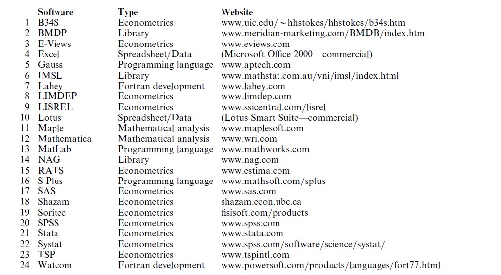
In an econometric analysis, the information in a data set which may include thousands or millions of values is distilled to a few equations which are claimed to describe the DGP. The intricacy of modern econometric techniques makes essential elaborate software with capabilities that extend well beyond the ubiquitous spreadsheet programs such as Excel (4) and Lotus (10) (which would be the nearest cousins to the software considered here). (Numbers in brackets refer to the list of computer programs in the Appendix.) Econometric software is used most frequently for the manipulation of large amounts of measured data for the purpose of constructing the equations that are the model of the process which produced the data.

2. The Evolution Of Econometric Software

The earliest software in econometrics was single purpose sets of Fortran language (‘Formula Translation’) code. The researcher who needed a program for a particular purpose would typically write it, or borrow it from someone else. One can find some of these programs in the appendices in some of the classic pieces in the literature, such as Nerlove and Press’s (1973) development of the multinomial logit model, the first edition of Draper and Smith’s (1981) exposition of regression analysis, Zellner’s (1971) early work on Bayesian estimation, and, more recently in Kalbfleisch and Prentice’s (1980) work on survival modeling. A typical journal treatment is Krailo and Pike’s (1984) exposition of a logit model for panel data, which contains a Fortran program listing for a standalone estimation program. Until the late 1960s, the journal Econometrica occasionally would publish short articles documenting computer programs developed by the authors.

2.1 Program Libraries

The process of building applications from scratch was made easier by ‘libraries’ of interchangeable parts for software development. The precursor to a very large group of programs currently distributed as the ‘BMDP Library’ (2) was a group of individual routines developed at UCLA in the 1960s under the heading of the ‘BMD’ (BioMedical) programs. These special purpose routines included subroutines for linear regression, Spearman rank correlation coefficients, cross tabulations, and so on. The BMDs initially existed as boxes of 80 column punched cards of Fortran code in the drawers of statistics labs. They maintained a common structure that allowed authors to write their own data setup programs to ‘plug into’ the package. Another programmer’s toolkit that was circulated widely in the 1970s was the ‘IBM SSP’ (Scientific Subroutine Package) which was part of the documentation for IBM mainframe computers. This book contained Fortran and C listings of programs for such functions as inverting or decomposing a matrix, and computing a variance. (‘C’ does not stand for anything. It was simply an extension of ‘B,’ itself a derivative of ‘BCPL’ (the BC programming language) and a contemporary of APL (a programming language). All were languages originally written to work with the Unix operating system on DEC’s original PDP-11 computers.

Most of the difficult computations being done by econometricians at this time involved complex matrix algebra, data manipulation, and random number generation. A library of well-written subroutines combined with the efforts of the analyst was quite sufficient for application development. This approach to programming has not vanished from the landscape. The Numerical Recipes books (C, Pascal, and Fortran) by Press et al. (1986), contain the modern counterpart to the expertly written library of subroutines contained in the SSP. The BMD libraries still exist as the commercial BMDP (2) routines, and the IMSL programs (6) and NAG (Numerical Analysis Group) (14) routines are still used by scientific programmers and in the development of major software packages. (IMSL, itself, grew largely out of a public domain library of matrix programs, EISPACK/-LINPACK. These provided the backbone for many early matrix implementations. They have since evolved to the (still) public domain package LAPACK (www.scd.ucar.edu/softlib/LAPACK.HTML and, see also NetLib at ORNL).

2.2 Integrated Packages

Early econometrics programs were single purpose Fortran programs that users passed amongst themselves and which grew over time as they were extended. The concept of a multipurpose, integrated econometrics package emerged in mid-1960s in the form of three particular programs, TSP (Time Series Processor), the Troll system, and B34S (which began as BiMed34; see Stokes 1997). TSP (23) and B34S (1) have remained active and are still under development. The early incarnations of these packages were primarily devoted to different forms of linear regression and correlation, but they have grown into vast assemblages of hundreds of thousands of lines of code (still mostly Fortran). Development of today’s two largest commercial statistics and econometrics packages, SAS (17) and SPSS (20) also began at this time, though generally in social sciences other than economics and focused on techniques largely different from those of interest to econometricians. The demise of the distribution of custom written, single purpose software began in the 1970s with the emergence of TSP, SAS, SPSS, and so on.

2.3 Development Settings

With the exception of E-Views (3), which is a fairly recent arrival, and of the language platforms, MatLab (13), S-Plus (16), Gauss (5), Maple (11), and Mathematica (12), which are arguably successors to Fortran, most of the major packages in current use began development as part of a cottage industry in the 1960s and 1970s, usually by an individual or small team of innovators. This is a distinct difference from the contemporary, corporate route to major software development. The modern development centers, such as SAS, Inc. and SPSS, Inc. are creations of the 1980s and 1990s. Nonetheless, many of the programs listed in the Appendix to this survey continue to be developed by small numbers of statisticians and econometricians whose names would be recognized by practitioners (most likely in association with literature encountered as part of their graduate studies).

2.4 Programming Languages

Wither the primitive programming languages, Fortran and C? Fortran dominated the scientific computing landscape for nearly four decades until the early 1990s, and remains the language of choice for many scientific applications, e.g., in physics and astronomy. The practitioner interested in writing a Fortran or C program may use one of the development kits for the PC (Windows) setting, such as Lahey (7) and Watcom (24). Time-shared systems, such as Sun Microsystems, also provide Fortran and C compilers and program libraries as part of the operating platforms. These vendors have extended the lives of Fortran and C as numerical language platforms, but this style of programming is a dying art. For software developers, Fortran is giving way to C, for example, in the full conversions of RATS (15) and SAS (17) and in the mixed language construction of LIMDEP (8). Individuals doing custom numerical programming increasingly rely on Gauss and its counterparts, MatLab, etc.

Recent developer’s programming language implementations have gravitated toward the studio format. The studio platform consists of integrated tools for merging code in one or more languages along with numerous libraries and ancillary tools. The Microsoft Software Developers Kit (SDK) is a popular example. This approach to programming has become essential for the development of major programs. One of the very useful innovations is the seamless creation of mixed language (e.g., Fortran and C++) platforms that allow developers to exploit the best features of both these languages. The end result is that C, its successor, C++, and Fortran, continue to play a major role in the development of modern econometric software, but only in the laboratories of developers, rather than in the toolkits of practitioners.

2.5 The Internet

Finally, in what may be a surprise given the breathless surrounding hype, it appears that the Internet has had little or no impact on econometric software beyond facilitating the transfer of files, programs, and information. It is otherwise difficult to discern any ways in which the actual mechanics of econometric computing have been affected by the creation or expansion of the Internet.

3. The Characteristics Of Modern Software

The software used by modern econometricians is essentially of two types. Most empirical research is done using one of the large, integrated packages that contain collections of programs for a variety of models. In these programs, complicated models are built with single, compact instructions. If a technique has gained acceptance in the applied literature, then it will appear as an ‘option’ in at least some of these packages. In contrast, when a technique or model proposed by an econometrician involves new methods or novel kinds of computations, then it is not likely to exist yet as a feature in an existing estimation platform. The computational tools that this analyst needs will typically be developed using one of the more primitive programming languages, such as Gauss (5), MatLab (13), SPlus (16) or, at an even lower level, one of the native programming languages, Fortran or C++.

3.1 Packaged Expertise

The term canned routine has long been used for programs that embody the econometric expertise needed by users. Some have argued that the use of such software locks practitioners into a limiting set of models. While the argument may once have had some merit, the huge variety of techniques and the customizability provided by most large packages makes the criticism moot for current purposes. In addition, contemporary software is mature enough that developers have incorporated optimal algorithms that purists who mimic the textbook mathematical formulations might not use, or even be aware of. Least squares provides an excellent example. The analyst who writes his own program for linear least squares regression is likely to rely upon the textbook matrix formula, b =(X`X)<sup>-1</sup>X`y. But, this is not the most accurate method of computing a least squares coefficient vector. Many large packages use much more accurate techniques, such as QR and singular value decompositions that avoid inversion and moments accumulation altogether. For the individual researcher to develop complicated low level tools such as this may well be excessively difficult.

3.2 User Written Programs

The distinction between these two types of software is somewhat blurry since the programming languages are often distributed with packages of routines that have been written by expert users. In addition, developers of code for Gauss (5) and MatLab (13) often distribute their programs on the Internet simply by posting them on their own websites, perhaps along with the research report of which the software development was a part. For example, all the major integrated econometrics packages contain an estimator for the logit model for binary choice, whereas the Gauss user must program their own. However, so many widely distributed Gauss libraries of routines contain users’ versions of the logit program that for practical purposes, Gauss does contain a logit estimator. In the other direction, large integrated packages usually contain their own ‘programming languages,’ which allow the user to construct capabilities that are not already contained in the program. Thus, while a program such as SAS (17) may not contain a specific command for estimation of a certain kind of survival model, it does contain a programming language for matrix manipulation as well as a means for a user to access certain utilities such as a nonlinear optimization program. Thus, the SAS user can develop a new estimator within his familiar SAS platform. TSP (123), SAS (17), SPSS (20), Stata (21), Shazam (18), EViews (3), and LIMDEP (8) to name a few, are all large integrated packages that also contain extensive matrix and data manipulation languages and access to nonlinear optimization programs which allow users to extend the modeling capabilities of the package. Thus, software developers and their users have blurred the distinction between preprogrammed procedures and programming languages.

3.3 Application Studios

The modern applied econometrician will usually maintain a toolkit of software consisting of one or more large packages, and, for less frequent usage, a low level development kit such as Gauss or MatLab, or a Fortran compiler, such as Lahey (7). Developers, conscious of this and sensing an opportunity, have begun to gravitate to a developer’s studio format for econometric software. As noted, all of the large packages provide low to medium level programming capability. Current trends, such as EViews, LIMDEP, RATS, SAS, Stata, and TSP have brought the programming features closer to the front end of these large, high level packages and Gauss with its large, expanding, and widely distributed library is approaching the same format from the opposite direction.

3.4 Common Features

Most general, integrated econometrics programs are quite similar. The model building process dictates the design, and as in many settings, a standard has evolved naturally. The following functions will be found in all the integrated packages, and, over time, will be mimicked by the users of the language packages as they collect their own routines:

(a) Data input and transformation;

(b) Model estimation—the estimation of model parameters, usually of several types;

(c) Statistical inference—testing hypotheses and forming probabilistic statements about quantities of interest;

(d) Specification, testing, and iterative refinement of model specification;

(e) Manipulation of model results for forecasting and simulation;

(f) Graphics and display of results.

Programs differ in some features and there is some amount of specialization, but most or all of the preceding will be found common to all. (Reviews are regularly published, e.g., in the Journal of Applied Econometrics.) The second function listed is one of the major dimensions on which programs differ. For example, EViews and RATS are particularly oriented toward analysis of time series data, SAS and Stata are especially complete in their presentation of techniques used in biomedical research, and LIMDEP is best known for its selection of models for discrete dependent variables. (Markets being what they are, there is substantial and growing overlap of these features.)

3.5 Interfaces

The means of communication between the user and the software is the interface. In order to describe this, it is necessary to make a distinction between mainframe and ‘PC’ (desktop style) operation. A second distinction between ‘batch’ and ‘interactive’ mode use is also necessary. The two distinctions are useful for describing the way certain computer programs work, although both modes do appear in both settings. Econometric software design began on large time shared mainframe systems. The design of such systems necessitated a batch mode form of interface. In this case, the user submits a set of instructions to a computer (operator, real or virtual) and returns later to retrieve their desired results. Modern computing carried out on the desktop, in contrast, usually involves an individual operating their own system interactively in the fashion of a large calculator, submitting single instructions (perhaps in the form of mouse clicked selections from menus) and instantly receiving the results of their directive. Econometric analysis often requires a hybrid of these two modes. Many estimation problems require huge amounts of computation that may take hours or days to complete, or lengthy scripts of operations. As such, a batch mode of operation is often necessary, even on a desktop computing platform. Therefore, there is normally some means of giving the program a directive equivalent to ‘carry out the following sequence of commands,’ or ‘fetch the set of commands contained in a certain file on disk and carry them out.’

There is a qualitative difference in the typical look and feel of a desktop computer compared to a timeshared mainframe. Modern desktop software is based on graphical user interfaces (GUIs). The amount of menuing varies from one program to another, but all modern econometrics programs are based on the GUI format. In contrast, there is relatively little GUI in the time-shared environment. The distinction is only superficial, however. The numerical functionality of most econometric software is easily replicated in both mainframe and microcomputer environments (e.g., all of the econometrics programs listed below except EViews). This is one of the strong distinctions between econometric software and, say, the programs used for graphics design or word processing. In the final analysis, the purpose of most econometric software is numerical analysis that can be done equally well in batch or interactive mode.

3.6 Estimation Procedures

To describe some of the remaining features, it is convenient to define some terms. Estimation is a process of culling from a data set a set of statistics that summarize the process by which the data were created. Estimation results range from single numbers, such as the parameter β in our earlier demand equation example, to one to one transformations of the original data, such as a periodogram, nonparametric hazard function, or kernel density estimator. Econometric software will contain ‘estimation routines.’ The term derives from the earliest days in which Fortran ‘subroutines’ were written for these purposes. The estimation routine consists of a body of code written to be invoked with a simple ‘command’ and provided with the specifics of a user’s problem. The command itself or the broader context of use of the software must define the kind of model to be estimated. Commands might be of the form ‘Using the data on Price and Quantity, fit a linear regression model.’

For example, one popular program, LIMDEP, uses the following, fairly typical style:

Regression ; Lhs=Quantity ; Rhs=One,Price $

that states in words that the user wishes the program to compute the constant term (ONE) and slope in a linear regression of quantity on price, Q=α+βP+ε. All integrated packages have counterparts to this kind of command, which is provided to the program by means of some kind of text processor. Some packages provide the same functionality by asking the user to select the estimation framework, then the variables in the equation from menus, instead. Many programs also allow users to choose either mode of entry. Each has its virtues—the former allows recording of steps and reuse of commands whereas the latter is generally more convenient.

A programming language such as Gauss would not contain such a broadly defined procedure. Rather, the Gauss processor would allow the user to define, using matrix expressions, the algebraic steps involved in doing the computation, including how to compute the coefficients for the model and how to compute certain statistics that the integrated processor would produce automatically. The user would then use the language’s built-in functions for displaying the results of their computations. Thus it would seem that a great deal more work is required of the Gauss user than the LIMDEP user. There is, but two issues motivate the former. First, as noted, many such sets of computations already exist, in elaborate routines that programmers have written and disseminated, so that these procedures can be used, often with a single command. Second, many estimation techniques do not exist (yet) in large integrated packages, so this is the only way to proceed. (Since this market is fast moving, it would be inappropriate to mention specific techniques. By the time this research paper appears in print, the information will be out of date.)

The remaining functions involve manipulation of model results. Some of these are handled automatically by the software while others must be assembled by the user. At this juncture, the user of the integrated procedure is likely to use some of the programming features of the package, such as a matrix computation. For example, the literature often produces new statistics or ways to manipulate the results produced by familiar models such as the linear regression model. The SAS, Stata, or TSP user is likely to handle this situation by constructing a ‘procedure’ with ‘adjustable parameters’ that might appear as follows:

‘Procedure: Regression;

Dependent variable is (Y), Independent variables are (x1, x2 )

Compute residuals as variable (e).

Compute and report statistics using

procedure …

End of Procedure’

Now, to invoke their procedure, the user might use a single directive such as:

‘Use Regression Procedure (Quantity, One, Price).’

The generality of the procedure allows it to be used for different problems just by changing the ‘call’ statement. At this point, the only difference between Gauss and SAS is the detail that will have to be programmed in the first line of the procedure.

3.7 Accuracy

One might think that given the textbook formulas for the necessary computations, all programs would get the same right answer for any particular problem. But, in fact, this is far from correct. Even in the absence of programming errors, there are large differences in the algorithms and methods used in computer packages. For practical purposes, two approaches are used for validating econometric software: replication and benchmarking. The first of these is strictly pragmatic. For most techniques, there are no applications with known correct answers against which to benchmark a program. As such, it is assumed that if two or more of the major programs give the same answer for a problem, then they both have it right. If they differ, then the tricky issue arises as to which, if either is correct and, again, the issue would have to be resolved in ad hoc fashion. A contemporary study that pursues this line of inquiry is Silk (1996), whose review of estimators for simultaneous equations models presents some surprising differences (see, also, McCullough and Vinod 1999.) The same approach has been taken in a review of programs for the computation of GARCH models by McCullough and Renfro (2000).

True benchmarking is now available for many common calculations. The tradition in econometrics begins with Longley’s (1967) true results to 10 significant digits for a specific problem in linear regression. The Longley standard was used for many years as the yardstick for linear regression programs; if a program could match the Longley benchmark to at least eight digits, then it could probably rise above suspicion for practical usage. Later analysis has showed that the Longley hurdle is not particularly high, and clearing it is not all that difficult, even for fairly mediocre software. The Statistical and Engineering Division of the National Institute of Standards and Technology (NIST) has published (www.nist.gov/itl/div898/strd) a suite of 57 benchmark problems in four classes: univariate statistics, analysis of variance, linear regression, and nonlinear regression. The NIST problems have been solved using very high precision methods, and correct answers have been published. In detailed reviews, McCullough (1998, 1999) found fairly wide differences in the performance of several econometrics packages. Since econometrics programs tend to be revised, refined, and updated very frequently, these differences are likely no longer to be evident by the time this research paper is in print.

4. The Role Of Software In The Development Of Econometrics

A convincing case can be made that several parts of modern econometrics awaited the development of software to gain currency.

In primitive incarnations, econometric software operated on a table of data with variables in columns numbered from left to right. To communicate a desired computation to a program, the user would specify columns of the table, as in ‘Regress the variable in column 5 on a constant, and the variables in columns 6, 8, and 10.’ TSP was among the first to allow names for variables to appear in a symbolic instruction to the program. The software went an important step further in that it allowed the components of equations to appear symbolically in words and familiar algebraic symbols. Software had begun to evolve in this direction, but TSP brought the language of equation specification up to the level of compilers such as Fortran. This major innovation changed the standard for econometric estimation programs.

The most important single development in practical econometrics in the period prior to 1970 was arguably the LSQ (Least Squares) procedure in TSP. The combination of symbolic equation specification with TSPs LSQ procedure allowed the birth of a very large literature on linear and nonlinear equation systems. The seemingly unrelated regressions model had been proposed a decade prior by Zellner (1962) and Theil (with Zellner, 1962), but the model did not appear in wide use until the appearance of LSQ. The procedure went an important step further in that it allowed the Zellner estimator to be extended to nonlinear systems of equations.

At roughly same time, Joreskog proposed a maximum likelihood approach to factor analysis and the estimation of general linear equation systems. The analytic results had been known for some time, but solvers for the likelihood equations for a general hierarchical linear equation system had not been widely distributed. Joreskog’s (1970) early work included ‘A Computer Program for Minimizing a Function of Several Variables,’ (Educational Testing Services: Research Bulletin 70-14). In this was published the numerical engine of a package published two years later as ‘LISREL’ (Linear Structural Relationships—originally, ACOVS for Analysis of Covariance Structures). ETS 70-14 contained a listing of Fortran computer code for optimization, including a very clever and effective technique for the line search step in optimization. LISREL spawned a very large and still growing industry in structural equations analysis in the social sciences. The technique is a major part of the methodology; the program, itself, has become Scientific Software, Inc. (9).

Of somewhat more recent vintage, is Heckman’s (1979) sample selection model. Building on his work on labor supply models, Heckman proposed a method for a regression model with a particular type of nonrandom sampling in a seminal paper in 1979. The computations involved are now fairly routine and incorporated in most econometrics packages, but in the mid-1980s, the technique became a standard tool in the microeconometricians kit as the LIMDEP program (8) became the de facto standard approach for implementing it.

The work of Sims (1977), Granger (1969), and Litterman (1986) in the mid-1970s on vector autoregressions (VARs) in econometric time series analysis produced a new body of theory to challenge the structural simultaneous equations models. The RATS (Regression Analysis of Time Series) (15) computer program, developed by these authors carried the methodology into the mainstream of applied econometrics. The development has also been ongoing, both of the program (Estima, Evanston, IL) and of the methodology as can be seen in any reference on time series, such as Hamilton (1994). (RATS has recently spawned CATS—Cointegration Analysis of Time Series.) Once again, the computations and the methods are not overly difficult, but the fact that they have been conveniently integrated into a general-purpose package has been an important impetus to the dissemination of the methodology in the applied literature. RATS was also an early contributor among several that significantly advanced practice by providing the user with access to an optimization program that required only a basic, again symbolic, specification of the problem. This freed the researcher from having to learn a large amount of programming. Contemporary programs, e.g., TSP, LIMDEP, and SAS, still RATS, Gauss, and so on, all offer this capability.

The earliest work in applied econometrics required the analyst either to use someone else’s program or to know how to write their own Fortran code. The latter type were in a distinct minority, so most researchers used software written by others. Current practice and contemporary software make it possible for researchers to choose among a vast array of prepackaged techniques and, with the aforementioned MAXIMIZE capabilities and the matrix programming languages of Gauss, B34S, LIMDEP, RATS, and so on, to create another vast array of extensions with easily acquired programming skills. The result has been an explosion in the variety of techniques and model formulations found in the published research.

5. Conclusion

The development of software has been a facilitator, and a platform for the dissemination of results and continued research in econometric techniques and methodology. But there are cross-currents in contemporary software design. As of 1999, econometric software design and publication has left the cottage industry of the 1960s and 1970s far behind; it is usually (though not always) a corporate endeavor. At the same time, technique, development, and extension of econometric methodology remain the bailiwick of a scientific community which has, to some extent, preserved the distinction between the purely commercial nature of, for example, the word processor market and the romantic, if antiquated, free exchange of scientific software among individuals and small teams of researchers. However, market competition appears to be working smoothly in the right direction, and no case could reasonably be made that market forces have inhibited the development of econometric techniques or software in the way they have, e.g., in the markets for operating systems and Internet browsers. Technological advance in software and econometric technique appears to be rapid and uninhibited.

Bibliography:

1. Draper N R, Smith H 1981, Applied Regression Analysis, 2nd edn. Wiley, New York
2. Granger C 1969 Investigating causal relations by econometric models and cross-spectral methods. Econometrica 37: 424–38
3. Hamilton J D 1994 Time Series Analysis. Princeton University Press, Princeton, NJ
4. Heckman J J 1979 Sample selection bias as a specification error. Econometrica 47: 153–61
5. Joreskog K, Gruvaeus G 1970 A computer program for minimizing a function of several variables. Educational Testing Services, Research Bulletin Number 70-14
6. Kalbfleisch J, Prentice R 1980 The Statistical Analysis of Failure Time Data. Wiley, New York
7. Krailo M, Pike M 1984 Conditional multivariate logistic analysis of stratified case-control studies. Journal of the Royal Statistical Society, Series A-Statistics in Society 84: 95–103
8. Litterman R 1986 Forecasting with Bayesian vector autoregressions—five years of experience. Journal of Business and Economics Statistics 4: 25–38
9. Longley J 1967 An appraisal of least squares programs from the point of the user. J. American Statistical Association 62: 819–41
10. Maddala G S 1983 Limited Dependent and Qualitative Variables in Econometrics. Cambridge University Press, New York
11. McCullough B D 1998 Assessing the reliability of statistical software. Federal Communications Commission, manuscript
12. McCullough B D 1999 Econometric software reliability: Reviews, LIMDEP, SHAZAN, and TSP, Journal of Applied Economics 14(2): 191–202
13. McCullough B D, Renfro C 2000 Benchmarks and software standards: A case study of GARCH procedures. Journal of Economics and Social Measure, in the press
14. McCullough B D, Vinod H D 1999 The numerical reliability of econometric software. Journal of Economic Literature 37: 633–65
15. Nerlove M, Press S 1973 Univariate and multivariate log–linear and logistic models. RAND -R1306-EDA NIH, Santa Monica, CA
16. Press W, Flannery H, Teukolsky S, Vetterling W 1986 Numerical Recipes: The Art of Scientific Computing. Cambridge University Press, Cambridge
17. Silk J 1996 Systems estimation: A comparison of SAS, Shazam, and TSP. Journal of Applied Economics 11: 434–50
18. Sims C 1977 Exogeneity and causal ordering in macroeconomic models, New Methods in Business Cycle Research: Proceedings from a Conference, Federal Reserve Bank of Minneapolis, MN, pp. 23–43
19. Stokes H H 1997 Specifying and Diagnostically Testing Econometric Models, 2nd edn. Quorum Books, Westport, CT
20. Zellner A 1962 An efficient method of estimating seemingly unrelated regressions and tests of aggregation bias. Journal of the American Statistical Association 57: 500–9
21. Zellner A 1971 Introduction to Bayesian Inference in Econometrics. Wiley, New York
22. Zellner A, Theil H 1962 Three Stage Least Squares: Simultaneous Estimation of Simultaneous Equations. Econometrica 30: 63–8