Aggregate Expenditures Research Paper

• Consumption expenditures are expenditures on final goods (excluding housing) and services by consumers, produced during the accounting period and in the economy under study.
• Investment expenditures are final goods and services purchased by businesses and buyers of homes, produced during the accounting period and in the economy under study. They include nonresidential structures of all types, plus all producers’ durable equipment, plus residential structures, plus all inventories produced in the accounting

period (some of these inventories may be planned, or desired, inventories; others may be unplanned, or undesired, inventories—unplanned inventories being acquired when sales are less than anticipated). Investment expenditures do not include financial transactions such as the purchase of stocks and bonds.

• Government expenditures are final goods and services purchased or produced by governments at all levels, produced during the accounting period and in the economy under study.
• Net exports are exports of final goods and services by the country under study (produced during the accounting period in the economy under study), minus the imports of such goods into that country.

The sum of these four spending components equals AE. AE thus equals GDP. That is, the total value of expenditures on final goods and services is equal to the total value of all that which is expended on the acquisition of final goods and services (i.e., GDP).

Theory

Expenditures, Planned Expenditures, and Inventory Adjustment

There are, however, two variants of the AE concept: actual AE, as defined previously, and planned AE. The latter is of particular importance in modern macroeconomics. Planned AE is the amount of expenditures the economy generates when all purchasers purchase an equilibrium amount of goods and services. It describes a state where purchasing decisions are consistent with the resources and needs of purchasers. (Planned AE often is referred to as aggregate demand.)

By way of illustration, consider the behavior of a typical retailer. Each month (let us say), a retailer assesses the state of its business and, based on that assessment, orders a particular quantity of the goods that it is its business to sell. At month’s end, any of the ordered goods that are unsold will be added to inventory. If the retailer’s assessment of the market demand for its product is correct, its sales of goods will be such that, at month’s end, it will be left with just the amount of inventory stocks on its shelves that is consistent with its long-run needs (needs given by relatively stable factors like how many customers the store loses if it runs out of goods its customers wish to buy, the financing costs of carrying such goods, etc.).

Suppose, however, that the retailer has overestimated the demand for its goods, so that it is left at month’s end with more unsold goods than it had expected. Had the store known, at the beginning of the month, that demand would be lower, then it would have ordered fewer goods. However, because it did not know this and so did not reduce its orders, some of the goods it had planned to sell to customers that month remain on the store’s shelves at month’s end. The retailer’s actual expenditures on new inventory for the month, then, are greater than its planned expenditures on inventory. The store’s actual expenditures on inventory now exceed what it would have spent if it had predicted monthly demand correctly. As a result of its miscalculation, the retailer now has excess, or unplanned, quantities of inventories on its shelves.

As an aid to clarity, consider a simple numerical example. Suppose a T-shirt retailer orders 100 shirts, planning to sell 80 and retain the other 20 as inventory. At month’s end, it turns out that the retailer has been able to sell only 70 of the 100 T-shirts that were ordered on the first of the month. It will, therefore, add the remaining unsold 30 T-shirts to its inventory, including 10 more than the 20 shirts it had planned to add. Had the store known that T-shirt demand would drop by 10 units, it would have cut its orders by 10 units, so as not to add more T-shirts than planned to its inventory stocks. Thus, had the retailer been fully informed at the start of the month about the state of demand for its product, it would have ordered only 90 T-shirts.

As things stand, the retailer has ordered 100 T-shirts when, had better information been available at the start of the month, it would have chosen to order only 90. The store’s planned investment is the 20 T-shirts it had planned all along to add to its inventories. Its unplanned (or involuntary) investment is the 10 T-shirts it adds to its inventories unintentionally. (Quite likely, next month the store will reduce its orders in order to “work off” its excess stock of inventories, weakening thereby the amount of economic activity at the factories from which it orders its stock of goods.)

The same type of reasoning, but in reverse, holds when the store finds that demand for its T-shirts is greater than expected. Suppose the store has ordered 100 shirts, again expecting to sell 80 and retain 20 as inventory. Suppose demand is greater than expected, equaling 90 T-shirts. The store will then sell all the T-shirts (80) that it had ordered for sale during the month. However, in addition, it will sell 10 more units that it had been planning to add to its stock of T-shirt inventory. The store’s planned investment is still 20 T-shirts, but its unplanned investment is -10 (negative 10) T-shirts, due to its unexpectedly strong sales. As a result, at month’s end, the store’s total investment is 10 T-shirts smaller than had been planned. (Quite likely, next month the store will increase its orders to increase its stock of inventories to its planned levels, increasing thereby the amount of economic activity at the factories from which it orders its stock of goods.)

The simple inventory problem faced by our retailer turns out to be quite important, both as a part of macro-economic analysis and in the actual economy. The economy often behaves as suggested in the retailer example. In periods of unexpected demand weakness, the economy’s retailers, wholesalers, and so on accumulate positive levels of unplanned inventories. Subsequently, retailers and other sellers of goods cut back on orders, causing less production upstream in the factories and so amplifying the initial weakening of the economy. In the reverse case, an unexpectedly strong economy causes an undesired depletion of inventories (negative levels of unplanned inventories), causing increases in orders at the factories and so amplifying the initial strengthening of the economy.

Another reason why the simple inventory problem is particularly important to macroeconomics stems from a characteristic of NIPA accounting. Consider consumption expenditures. How much of the spending that consumers do is truly intended or planned, and how much of it is mistaken (i.e., with full knowledge, particular consumers might have bought more, or less, product than they did in fact buy)? Because of the inherent impossibility of making such a determination, NIPA accounting simply assumes that all of the spending carried out by consumers is planned spending. Similarly, all government spending is considered to be planned spending, and the same convention is applied to net exports. However, for the case of investment spending, as we have already seen, planned expenditures and actual expenditures do differ. In fact, it is in the investment spending accounts that all of the gap between AE and planned AE is found. When consumers, governments, or “net exporters” unexpectedly reduce their expenditures, all of the goods they have chosen not to purchase wind up being held as inventory by merchants who were unable to sell these goods (and vice versa if spenders unexpectedly increase their expenditures). The distinction between planned and unplanned inventory stocks, therefore, is the mirror image of unexpected changes in expenditures by others in the economy.

Planned AE and Inventory Adjustment: The Keynesian Cross

The preceding analysis suggests a simple visualization of macroeconomic fluctuations, based on firms’ inability to consistently predict demand and the resulting accumulation or reduction of inventory stocks on the firms’ aggregate balance sheet. Consider a substantial and unexpected reduction in planned AE in an economy that has grown accustomed to a higher level of such expenditures. As a result, sales fall, and unplanned inventories accumulate on firms’ shelves and in their warehouses.

How will retailers, wholesalers, and so on react to the undesired swelling of their inventory? There are two possibilities, in principle. One is for them to immediately lower their prices by enough to induce buyers to quickly clear out their excess inventory by taking advantage of these “fire sales.” However, because these firms will likely take a sizeable capital loss on their inventory stocks if they eliminate them in this way, they are often reluctant to lower their prices by enough to sell off very much of their excess inventory stock. The alternative strategy is to hold prices more or less unchanged and to reduce the size of their orders from the factories. This way, firms allow their excess stocks of goods to be worked off slowly over time (because business has slowed, this second strategy usually also involves laying off a portion of the firms’ workforce).

To an extent, firms will pursue both of these strategies. However, it is a common observation that firms primarily respond to excessive inventories by laying off workers, cutting orders, and working off inventory stocks slowly over time. This strategy, however, transmits weaker sales “upstream” to wholesalers and factories as described previously, triggering weaker economic activity in these sectors too and causing a lessening of activity and layoffs in those sectors. These layoffs, in turn, reduce demand by consumers in still other sectors where these consumers purchase items, triggering still more unplanned inventory buildup and layoffs in those other sectors, and so on (in a dynamic sequence commonly known as the multiplier process). Thus, the initial decline in planned AE that had initially led to firms’ accumulation of unplanned inventory investment can, through the preceding sequence, become a general decline in economic activity.

The standard graphical model used to illustrate this process is known as the Keynesian cross (after John Maynard Keynes, who founded this line of thought). Sometimes it is instead called the 45-degree line diagram (after the graph’s most notable visual feature). Before discussing this diagram, however, we need to clarify an important relationship in our simple model. One of the core principles of national income accounting is that, allowing for a couple of side issues, the production of a given dollar amount of GDP generates an equal dollar amount of income for the factors of production that participated in the production of that GDP. In fact, this statement is only an approximation of the true state of affairs, due to the side issues of depreciation expenditures and indirect business taxes. In the actual economy, before counting our new production this year, we must replace the equipment we used up (or depreciated) last year due to our productive activities then. Also, in the actual economy, there are indirect business taxes that tax away some business receipts before they can be distributed to the factors of production. However, in our simple illustrative economy, we ignore these two factors. An alternative treatment uses net national product (NNP), which is GDP minus depreciation expenditures, as the core national output concept (indirect business taxes are again set at zero). Using NNP as the output concept is more realistic than using GDP, because depreciation expenditures need not be assumed away as in the discussion in the main text of the research paper.

Returning to the main argument, in our Keynesian cross framework, every dollars worth of production generates exactly a dollar’s worth of income to those owning the factors of production. In the aggregate, then, national output (GDP) equals national income by definition. We will take this equivalency seriously, so much so that we will even use the same symbol Y to simultaneously represent both national output and national income. That is, in what follows, we will call Y either national output or national income, depending on which better fits the context.

Returning now to our main line of discussion, Figure 1 depicts the Keynesian cross diagram, which is interpreted as follows. Assume a simplified economy where all spending is done by either consumers, investors (the latter, recall, buy capital goods, not stocks and bonds), or governments. (There is assumed to be no trade with other nations, so that net exports are zero, a common simplifying assumption known as the closed economy assumption. We briefly discuss the effects of net exports on planned expenditures later in this research paper.) Consumers spend according to the Keynesian (linear) consumption function

C = a + bYD,

where C is expenditures by consumers. C depends predominately on income after taxes (YD) (or disposable income); “b,” a parameter known as the marginal propensity to consume, gives the rate at which consumption increases in response to a change in disposable income (0 < b < 1); “a,” a second parameter known as the autonomous level of consumption, captures the impact of all forces other than disposable income (such as expectations of the future, household real wealth, etc.) that affect consumption behavior (a > 0). It is traditional to convert the consumption function into a function of income before taxes (Y), and taxes, by introducing a simple tax equation into the discussion. Here we assume a proportional income tax system, so that T equals tY, where T is tax revenues, t is the income tax rate (0 < t < 1) and Y is income before taxes.

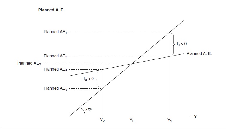
Figure 1   The Keynesian Cross Diagram

It is now traditional to assume a linear (or straight-line) consumption function, meaning that, whether income is high or low, the rate at which consumption increases with income remains the same. Keynes himself (1936/1965, pp. 31-32) and some of his followers emphasize the claim that the consumption function is nonlinear, flattening as income rises, so that consumption rises less and less per dollar of increased income as incomes rise. This notion is consistent with the claim that a society with higher income is inclined to spend proportionately less per dollar of new income, making the economy more dependent on investment and government spending if it is to reach full employment. However, many economists do not regard the nonlinearity issue as empirically significant. They prefer to use the linear consumption function, defending it as a reasonable approximation of reality that has the additional advantage of exploiting the flexibility of the linear functional form (vs. the more mathematically complex nonlinear functional form). The use of the linear form has important advantages. For example, strictly speaking, the marginal propensity to consume is defined only for very small changes in disposable income. However, if the consumption function is linear (as is assumed here), the same proportionate relationship holds for small or large changes in disposable income. We assume a linear consumption function throughout this research paper.

Substituting the tax equation into the consumption function and manipulating terms yields the revised consumption function,

C = a + b(1 -t)Y.

The advantage of this expression for present purposes is that it is expressed in terms that are easily portrayed on the Keynesian cross diagram (which measures real dollars of before-tax expenditure on its vertical axis, and dollars of real income, or output, on its horizontal axis).

The Keynesian cross diagram is designed to highlight, not the determinants of investment spending, but rather the consequences of changes in investment spending and government spending.

Accordingly, to describe the investment sector, let us take the simplest possible description of planned investment spending—one that assumes a given, exogenous level of such spending. Thus, the investment equation is

I = Io,

where I0 denotes a given level of planned investment expenditures. The interpretation here of investment spending as planned, not actual, spending is crucial. As described previously, planned investment expenditures are the level of investment expenditures such that businesses expect at the month’s close to end up with their planned (or equilibrium) levels of inventory stocks. The interpretation of I0 in this way means that our expenditures expression is one of planned AE, not actual AE, which, as discussed previously, equals national output by definition. Here it is also useful to recall that planned consumption expenditures equal actual consumption expenditures by definition, and planned government expenditures equal actual government expenditures by definition (the same is true for net exports in versions of the model where they are included).

Our third source of expenditures is government. Again, we make the simplest possible assumption about government spending, which is assumed to be exogenously given as

G = Go.

The equation for planned AE in this model is, accordingly,

planned AE = a + b(1 -1 )Y + I0 + G0 = [a + Io + Go] + b(1-t)Y.

The rightmost side of this expression is what is called in basic algebra the point-slope form. Therefore, the intercept term is [a + Io + Go], while the slope of the line equals b(1 -1). When we graph the planned AE expression on the Keynesian cross diagram, the intercept of the planned AE line is where that line intersects the vertical axis. At this intercept point, the value of planned AE equals [a + Io + Go], which is the amount of planned AE that corresponds to a Y level of zero (since people are earning no income at such a point, presumably they are living off their previous savings). Further, the slope of the planned AE line is b(1 – t). Planned AE increases with income due to the consumption function. For every dollar of increase in income, planned AE will increase by b(1 – t). For example, suppose that b equals 0.8 and t equals 0.5. Then b(1 -1) equals 0.4. Each dollar’s increase in income will create an additional 40 cents of planned AE (the reverse is true for one dollar’s decrease in income). The planned AE line always has a slope less than 1, due to the impact of the marginal propensity to consume and the income tax rate (because both b and t are fractions, their product will also be a fraction). So long as the vertical intercept of the planned AE line is positive (as seems reasonable), the planned AE line will intersect the 45-degree line at some point.

What notion of equilibrium is appropriate for this representation of the macroeconomy? One simple idea is that equilibrium be described as a state where total planned expenditures are just sufficient to purchase all of the economy’s output. This means that, in equilibrium, total planned expenditures equal GDP. It also means that planned investment expenditures equal actual investment expenditures. That is, inventories held by firms at the end of the month equal the inventories the firms planned to have when they placed their orders at the start of the month.

Strictly speaking, we are assuming that every firm has zero unplanned inventories. (In applying the framework to the actual economy, the corresponding assumption is that firms on average have inventory levels that are consistent with their planned levels.) All of the goods produced that month are being voluntarily consumed or held by some spender in the economy.

How will this reasoning play out graphically on the Keynesian cross diagram? (Please refer to Figure 1.) Notice first the interpretation of the 45-degree line that shoots out from the origin, cutting the graph in two. Because the vertical and horizontal axes are measured in the same units (real dollars of national output), the slope of this line equals 1, so that any point along it is a point where planned spending and national output are equal. That is, any point that rests on the 45-degree line is a point of potential equilibrium in the model. Which particular point is the point of equilibrium, however, will be determined by the level of planned AE that is generated by the economy’s consumers, investors, and local, state, and national governments. Equilibrium occurs precisely where planned AE intersects the 45-degree line, at the point where planned AE equals planned AE3 and Y equals YE. Only at this point is the amount of planned spending generated by the economy just equal to the amount of output produced by the economy.

To see further why this intersection is interpreted as a point of equilibrium, consider a point on the planned AE line that is associated with a Y level that is greater than the equilibrium point (Y = Y1 > YE). At output level Y1, the amount of planned AE needed to buy up all of the economy’s output is given by planned AE1—the planned AE level given by the intersection of the (vertical) Y1 line and the 45-degree line. However, the planned AE actually generated by the economy at Y1 (planned AE2) is given by the intersection of the Y1 line and the planned AE line. The amount of planned AE generated at Y1 is thus less than what is needed for equilibrium.

The deficiency of planned AE at Y1 will reveal itself in the form of unplanned inventory accumulation by firms (Iu > 0). (Iu can refer to either unplanned inventory accumulation or unplanned investment spending. This is because all unwanted investment takes the form of unwanted inventories.) Businesses, finding themselves holding more inventories than planned, will reduce their orders of goods. This in turn will reduce production at the factories, pushing the economy’s output leftward, away from Y1 toward the equilibrium value YE. So long as unplanned inventories are positive, this trend will continue until the economy’s output reaches the equilibrium point YE.

Now consider a point on the planned AE line that is associated with output level Y2, which is less than the equilibrium output YE (Y = Y2 < YE). At output level Y2, the amount of planned spending needed to buy up all of the economy’s output (planned AE5) is given by the intersection of the (vertical) Y2 line and the 45-degree line. However, planned AE actually generated by the economy at Y2 (planned AE4) is given by the intersection of the Y2 line and the planned AE line. Planned AE at Y2 is greater than what is needed for equilibrium. The excess of planned AE at Y2 will reveal itself in the form of unplanned inventory rundown (IJJ < 0; i.e., negative levels of unplanned inventories) on the part of firms. Firms, finding themselves holding fewer inventories than they had planned, increase their orders of goods. This in turn increases production at the factories, pushing the economy rightward toward higher output levels, away from Y2 toward the equilibrium value YE. So long as unplanned inventories are negative, this trend will continue until the economy’s output reaches the equilibrium point YE. Actions by firms to move their inventories to equilibrium levels is the primary mechanism driving the economy to its equilibrium on the Keynesian cross diagram.

While the preceding is the standard explanation of how equilibrium is reached on the Keynesian cross diagram, it is not necessary to rely on inventory adjustment to explain the move to equilibrium. In the mid-1980s, Robert Hall and John Taylor (1986) came out with a version of the Keynesian cross model that did not involve inventory accumulation and depletion. Their model, in brief, imagines a world without inventories of goods. Instead, firms “inventory” productive capacity by hiring workers who perform services for firms. An overly optimistic company will find itself with too many workers on staff. Productive capacity then exceeds the actual spending that the economy’s spenders are able to generate. The incomes of spenders are insufficient to support the current level of output. This puts downward pressure on the economy and tends to move output downward until the excess productive capacity is eliminated and equilibrium (which Hall and Taylor call spending balance) is achieved. Clearly, the model is not too different from the text’s inventories-based version, but, as the authors point out, it is useful to show that the mechanisms of the model do not depend on the existence of inventory accumulation in an essential way.

Applications, Refinements, and Policy Implications

Comparative Statics of the Keynesian Cross Diagram

The Keynesian cross diagram also can be used to show the impact on AE and equilibrium income of various changes on the demand side of the economy. Starting from the equilibrium position on Figure 1, consider, for example, a large, unexpected decline in planned investment. On the Keynesian cross diagram, such a change will shift the planned AE line downward (parallel to the original line). Once planned AE falls, YE will no longer be an equilibrium value. Unplanned inventory will accumulate on firms’ shelves. They will respond by cutting their factory orders, reducing production at the factories, and eventually bringing about a new equilibrium value at a smaller value of Y (to the left of the former equilibrium value, YE).

Can anything be done by government to counter such a decline in equilibrium income? In the Keynesian cross framework, the answer is an unambiguous “Yes.” The government has the two main tools of fiscal policy at its disposal: changes in government spending (G), and changes in income tax rates (t). By increasing G, the government can shift the planned AE line upward—in principle, by just enough to fully compensate for a decline in planned investment spending. The government may also cut income tax rates, increasing the slope (but not the intercept, given the assumed strictly proportional income tax system) of the planned AE line. The upward rotation by the planned AE line moves the economy’s equilibrium Y value upward and rightward along the 45-degree line. Either increases in G or decreases in t, or both, will increase equilibrium income, through our now standard mechanism of inducing changes in inventory accumulation (either causes inventory rundown). Retailers then increase their orders, increasing production in the factories and raising Y. The Keynesian cross diagram neatly illustrates the potential for activist government fiscal policies to counter undesirable changes in private sector spending.

Monetary policy’s impact also may be represented on the Keynesian cross diagram. A stimulative monetary policy— one that increases the money supply or its rate of growth— is commonly viewed as lowering the economy’s interest rates, which in turn triggers additional borrowing by firms, who then spend the money on new investment projects. The resulting rise in planned investment expenditures can be interpreted on the Keynesian cross diagram as an upward shift in the planned AE curve, which then stimulates the economy through the same inventory-based adjustment mechanism.

The “Open” Economy

The preceding discussion, for simplicity, assumes a closed economy—that is, an economy that does not trade with other nations. How do things change when trade with the rest of the world is introduced? Now, a fourth potential source of spending (which can be either positive or negative) is introduced: net exports. Net exports equal the goods and services that the economy exports to other nations of its production (exports), minus the goods and services that the economy imports from abroad (imports). When exports are greater than imports, then net exports are positive and planned AE is larger than in the case of the closed economy (the economy, in this case, is often said to be running a trade surplus). Citizens of other nations are adding to our economy’s domestic demand, causing planned AE to rise. Accordingly, when net exports are positive, the planned AE line shifts upward on the Keynesian cross diagram. By contrast, when exports are less than imports, then net exports are negative and planned AE is smaller than in the closed-economy case (the economy, in this case, is often said to be running a trade deficit). In this case, our economy, on net, is buying goods from abroad that often could be purchased domestically. Other things held constant, this means less demand for goods produced in our economy. Accordingly, when net exports are negative, the planned AE line shifts downward on the Keynesian cross diagram.

When net exports are included as a source of AE, the model is known as an open economy model. In the open economy, AE depends on the volume of net exports in two fundamental ways. First, an increase of income in the “home” country tends to increase the purchases of goods generally, including goods produced abroad. In the short run, this increase in home country spending increases imports into the home country without increasing exports (as incomes abroad are as yet unchanged). Thus, net exports decrease and, other things equal, planned AE in the home country declines. (In the event of a given fall in income, the effect is reversed.)

Second, a given increase in interest rates in the home country relative to abroad encourages a flow of investable funds into the home country. The process of investing these funds in the home country drives up the home country’s exchange rate, making home country goods more expensive to foreign citizens, and making foreign goods cheaper for home country citizens. Thus, exports fall, imports rise, and net exports fall, reducing the level of AE in the home country (other things equal). (In the event of a given fall in interest rates, the effect is reversed.)

Meaning of “Equilibrium” in the Keynesian Cross Diagram

The interpretation of the so-called equilibrium on the Keynesian cross diagram has been the subject of much controversy. Much of the controversy centers on the concept of full employment and the question of whether or not an economy could be in equilibrium without being at full employment. When economists speak of the full-employment position of the economy, they mean the economy’s maximum production level that is consistent with macroeconomic well-being. Too little production (i.e., an economy below full employment) means that the economy is not getting all the output out of its scarce resources that it should. Too much production (i.e., an economy above full employment) means that the economy is overheated. That is, the economy is producing at such a hefty pace that painful side effects like inflation and spot shortages of crucial raw materials (known as bottlenecks) are being created to an unhealthy degree. Above full employment, it is also possible for an economy to find itself destabilized, triggering a sharp decline in economic activity (even an outright recession).

In Chapter 3 of the General Theory, Keynes presented an aggregate demand and aggregate supply framework that later inspired the Keynesian cross diagram. Keynes emphasized that there was no particular reason why the equilibrium reached by the economy in his framework should correspond with full employment. Equilibrium could be above, equal to, or below full employment (though Keynes was quite sure that it would usually be below it; 1936/1965, pp. 118, 254). Keynes saw this equilibrium as a true point of stability—once reached, it would be hard for the economy to move itself away from it and to the economy’s full employment position. To classically oriented macroeconomists who criticized Keynes, the notion of a stable macro-economic “equilibrium” that was not at full employment was almost a contradiction in terms. (A lengthy debate about this and related matters dominated macroeconomics through much of the late 1930s and 1940s.)

When followers of Keynes such as Alvin Hansen and Paul Samuelson substituted the Keynesian cross diagram for Keynes’s framework, they kept Keynes’s sharp separation of equilibrium and full employment. Over time, however, macroeconomists grew increasingly uncomfortable with a notion of macroeconomic “equilibrium” that was not also situated at full employment (see, in particular, Patinkin, 1948, esp. pp. 562-564). As it had been before Keynes, price flexibility—a slow but still steady and substantial force in the economy—became again a generally accepted mechanism through which economies that were away from full employment were returned there. Many of Keynes’s successors downgraded the Keynes/Hansen/ Samuelson notion of equilibrium to the lower status of a mere short-run equilibrium. Long-run equilibrium was then defined in the traditional, classical economics manner as something occurring only at full employment.

The idea behind this divergence of equilibrium notions probably came from the microeconomics of Alfred Marshall. Marshall taught Keynes and doubtless influenced him in his decision to propose a short-run equilibrium concept in macroeconomics. In Marshall’s microeconomic theory of perfect (or pure) competition, the short-run equilibrium is defined for a case where the number of firms in the industry is fixed (there is not enough time for firms to enter or exit the industry). In the long run, when free entry and exit are allowed, a long-run equilibrium emerges that is quite distinct from the short-run equilibrium.

The macroeconomic version of the idea is that, while there are certain slow-acting forces that eventually move the economy to full employment, they are dominated in the short run by quicker acting forces. Chief among these slower acting forces is price level adjustment. In theory, it alone is sufficient to eventually move an economy to the full employment position. However, in the short run, the economy’s price level moves little, so that it can safely be assumed to be constant (or “sticky”). Based on such reasoning, a macroeconomic short-run equilibrium exists that is reached not through price changes but rather through changes in quantities—such as the inventory adjustment mechanism described previously. Thus, the argument concludes, a short-run model ought to emphasize planned AE and its determinants and place little emphasis on full employment, while a long-run model of the economy ought to emphasize full employment and to de-emphasize traditional Keynesian notions in favor of more “classical” ones.

More recently, the equilibrium notion in the Keynesian cross diagram has been downgraded even further into a mere “spending balance” (see Hall & Taylor, 1986, or a more recent edition of the text, such as Hall & Papell, 2005). Hall and Taylor divorce the model from its longstanding equilibrium connotation, even to the point of denying to it the term itself. The idea is that the intersection of planned AE and the 45-degree line represents a balancing point for the economy, which the economy reaches quite quickly, but which should not really be conceived as an equilibrium per se because the balance point changes quickly whenever the level of (planned) expenditures alters. Hall and Taylor reserve the term equilibrium only for the full employment position, insisting that only after the price adjustment process has moved the economy to the full employment point can the notion of equilibrium be usefully invoked. The authors’ approach to interpreting the intersection of the 45-degree line and the planned AE line is in the spirit of modern treatments, which insist that the healing role played by price adjustment in macroeconomics be taken seriously, not suppressed, as in the Keynesian cross model.

Here it should be pointed out that Keynes and his immediate followers were thoroughly skeptical of aggregate price adjustment as a cure for recession. Keynes felt strongly enough about the issue to present a detailed critique of it as his first major topic in the General Theory. In a nutshell, Keynes and his followers emphasize how lower input prices brought about by price adjustment adversely impact incomes of those already employed. This downward push to demand could more than wipe out the supply-side gains from lower costs of production. For details, see Keynes (1936/1965, chaps. 2, 3, 20). Modern macroeconomics, as portrayed in the Principles textbooks (e.g., McConnell, 1969), implicitly assumes that these adverse demand-side forces are dominated strongly by supply-side effects of lower input prices. Later versions of Keynesianism present arguments backing up the assumption (see, e.g., Snowdon & Vane, 2005, pp. 114—116).

Strengths and Weaknesses of the Keynesian Cross Model

Since its origination in the 1930s and 1940s by Keynes, Hansen, and Samuelson, the Keynesian cross model has been a durable workhorse of macroeconomics. Its primary strength is its highlighting of inventory adjustment as a crucial part of the short-run aggregate adjustment process. There is little doubt that incomplete inventory adjustment and the changes in output that such incomplete adjustment calls forth makes a significant contribution to short-run aggregate fluctuations. The financial press routinely refers to an inventories-driven business cycle that has contributed to cyclical movements in the post-World War II era (see, e.g., Gramm, 2009). The Keynesian cross framework captures these important real-world forces neatly in one tight diagram. As such, it is a useful tool for teaching about one of the core short-run adjustment processes of the macroeconomy (inventory adjustment) and its aggregate consequences.

That having been said, the model is not without its weaknesses. The most glaring is that prices in the model—including inventory prices—are fixed exogenously outside of the model. Consequently, one of the most fundamental mechanisms in economics—the tendency of surpluses to be eliminated by price declines, and vice versa—is not allowed to function in the Keynesian cross framework. Moreover, there is no link between the inventory adjustment process and aggregate price determination in the model. The constant-price assumption has been a significant, and much criticized, feature of many Keynesian models (particularly those dating from the early years of Keynesianism). The Keynesian cross diagram is an excellent example of such a model. Keynesians can, and do, respond that the time period of analysis assumed in the Keynesian cross model is too short to allow meaningful price adjustment. Keynesians can also cite plausible reasons why various prices should be “sticky” over short periods of time. However, the notion that price adjustment does not play at least some role in firms’ elimination of stocks of unplanned inventories is, to many economists, counterintuitive. The best that can be said on this point is that the Keynesian cross model should be conceived as an exploration of the aggregate consequences of inventory adjustment subject to the assumption that prices are fixed. (Some additional criticisms of the Keynesian cross framework are discussed in Weintraub, 1977, and Guthrie, 1997.)

This criticism applies mainly to the Keynesian cross diagram as a stand-alone model. The model works better when conceived as an “input” into what Hall and Taylor (1986) have called the aggregate demand/price adjustment model. In this framework, the role of the Keynesian cross diagram is mainly to help generate the so-called IS curve, which gives an equilibrium relationship between various interest rate levels and planned AE. The IS (or “investment = savings”) curve gives all the equilibrium points relating the interest rate and real income for a given set of model “parameters.” It is drawn on a graph with the interest rate on the vertical axis and the level of real income (or real output) on the horizontal axis. The IS curve is downward sloping, reflecting how a higher interest rate drives down planned investment spending and thus lowers the economy’s equilibrium income (and vice versa). The IS curve is commonly derived graphically from the Keynesian cross diagram. On the Keynesian cross diagram, a rise in the interest rate shifts the planned AE line downward (and vice versa). The derivation is done as follows. First, make an empty graph with the interest rate on the vertical axis and real income (or real output) on the horizontal axis. Second, place that graph directly above a Keynesian cross diagram. Because real output is on both horizontal axes, the two graphs “line up” vertically. Third, vary the interest rate, observing the resulting values in equilibrium income that are generated on the Keynesian cross diagram. Finally, derive the IS curve by plotting this relationship between the interest rate and equilibrium income onto the upper graph.

Once it is derived, the IS curve is combined with a Liquidity = Money Supply (LM) curve and a price adjustment equation to create a general model of the expenditures side of the macroeconomy. The IS/LM graph in turn can be used to generate an aggregate demand curve, which relates various values of the price level to planned AE. Then, this aggregate demand curve is combined with a supply-side model to give a general macroeconomic model of the aggregate economy. This model incorporates everything from the macroeconomic consequences of deviations in planned investment spending (including planned inventory spending) and other demand-side changes, to the macroeconomic consequences (and causes) of supply-side forces and price level changes. Numerous additional important topics can be analyzed as well within this broader framework.

Historical Development of the AE/Keynesian Cross Framework

Development of the Planned AE (Aggregate Demand) Concept

While the Keynesian cross framework emerged out of the Keynesian revolution, many of the ideas behind that model are far older than Keynesianism. Planned AE was called effectual demand, effective demand, or purchasing power in pre-Keynesian days. Even as early as the eighteenth century, the mercantilist school emphasized what Keynes (1936/1965) later called “the great puzzle of effective demand” (p. 32; see also his chap. 23). Most leading classical economists downplayed the notion of deficiencies in planned expenditures (or aggregate demand, as planned expenditures were usually called at the time). They believed that, except for brief and self-correcting “crises,” planned AE would take care of itself so long as production was unfettered and the types of goods produced were consistent with what consumers wanted and were able to purchase. Thomas Malthus, a notable exception, insisted that an economy could have serious drawn-out problems with inadequate effective demand (his arguments were a regular bone of contention in the early nineteenth century between himself and David Ricardo, a key founder of classical economics). Keynes lauds Malthus’s position and writes also of how, during the heyday of the classical school, ideas that took effective demand failure seriously “could only live on furtively, below the surface, in the underworlds of Karl Marx, Silvio Gesell or Major Douglas” (p. 32).

Like Keynes, early anticlassical thinkers were concerned mainly with the prospect of secular (long-term) demand failure—not just with occasional downward fluctuations in planned AE that contributed to a downward swing in the business cycle. Keynes saw the laissez-faire macroeconomy as routinely—not just occasionally— underperforming its potential due to problems with generating sufficient levels of planned expenditures (see, e.g., Keynes, 1936/1965, chap. 1; chap. 3, p. 33, bottom paragraph; chap. 12, p. 164, final sentence; chap. 18, p. 254). There is also the fact that Keynes chooses to develop a business cycle theory only at the end of the book (chap. 22). If the General Theory were primarily about combating the business cycle, purely cyclical forces surely would have been given a more prominent role in the main portion of the volume.

Keynes’s (1936/1965) chief (though far from sole) culprit causing inadequate AE was unstable confidence by the business investment sector, which created secular underinvestment and thus routine unemployment problems (chap. 12). The worldwide Great Depression, which raged even as Keynes was writing his famous General Theory, seemed thoroughly consistent with Keynes’s analysis. Never before had the hypothesis of secular effective demand failure seemed so confirmed by day-to-day events.

This certainty, however, faded with time in the post-World War II era in the face of a recovered economy and a withering fire by the inheritors of the classical tradition. Since Keynes wrote, the “market failure” interpretation of the Great Depression has been effectively challenged by the heirs of the classical tradition. The most famous example is Milton Friedman and Anna Schwartz (1963; see also Friedman & Friedman, 1980, chap. 3), which emphasizes an unprecedented contractionary monetary policy during the crucial 1929 to 1933 period. Others have focused on the extraordinary uncertainty created by government actions during the decade of the 1930s (see Anderson, 1949; Smiley, 2002; Vedder & Gallaway, 1993).

It is a common misconception that the classical economists of the late eighteenth and early nineteenth centuries, as well as the early twentieth-century heirs of the classical tradition, had no interest in, or theory of, planned AE. Indeed, this is arguably a fair assessment of some classical writers. However (though the term itself was not used), short-term declines in planned aggregate spending were seen by several classical economists as being a key part of every business cycle downturn (or crises, as they were called at the time). Classical economists, however, differed from Keynes in two significant ways. First, they flatly rejected any notion of secular failure in planned AE. Second, they did not see declines in planned expenditures as being the ultimate cause of recession. Instead, they saw these declines as being caused by other more fundamental factors (such as disruptive government regulatory, or monetary, policies). Even before the classical era, David Hume (1752/1955, pp. 37-40) presented a very modern tale of a recession being caused by an unexpected decline in the money supply. Nearly a century later, John Stuart Mill (1844/1948, esp. pp. 68-74) described how a crisis of confidence could cause people to hoard money and so reduce their purchases of goods. Allowing for the difference in vocabularies between his time and ours, Mill accurately described such an episode as being caused by a short-term decline in planned AE (or aggregate demand).

Early twentieth-century macroeconomists (whom Keynes, peculiarly, also labeled classical) also focused on aggregate demand issues—though always in the context of trying to understand cyclical, rather than secular, fluctuations. Leland Yeager (1997) summarizes numerous early twentieth-century business cycle theories that accurately identified the demand-side forces at play in the downturn— although such a downturn in demand was seen routinely as the effect of still more basic forces (such as a decline in the money supply). J. Ronnie Davis (1971) details how economists in the 1930s at the University of Chicago and elsewhere pursued lines of thinking parallel to Keynes’s, suggesting that Keynes’s ideas were “in the air” at the time.

Still, despite these glimmers from earlier scholars, it is without a doubt John Maynard Keynes who is primarily responsible for the ascendancy of demand-side macroeconomics through the influence of his General Theory (1936/1965). Keynes confronted a profession that took little explicit interest in the study of aggregate demand and left that profession positively consumed by the topic. Short-run macroeconomics, including the study of the business cycle, has since Keynes’s day placed great emphasis on questions pertaining to short-run planned AE. Through about 1976, the primary focus of macroeconomics was to examine the theory and determinants of planned AE (Friedman, 1968, is still the classic brief summary of much of the period covered in this section. It is highly recommended to the student’s attention). The main determinants of planned AE—consumption, investment, government, net exports, and the demand for and supply of money—the statistical properties of these components, and ways for the monetary and fiscal authorities to alter these aggregates are topics that have all been extensively explored. The profession’s comprehension of the practicality of the basic Keynesian policy agenda has improved markedly as all aspects of that agenda have been placed under the magnifying glass.

At the risk of some oversimplification, it may be said that two fundamental issues dominated the policy agenda of those who worked on developing the Keynesian framework in the 30 years following Keynes’s death in 1946. The first concerned mainly the channels and mechanisms through which demand-side policy worked, while the second focused on the relative strengths and weaknesses of fiscal policy (changes in government spending, tax-rate changes) versus monetary policy (changes in the money supply or in its rate of growth). Through this entire era, understanding was enhanced considerably by the development of statistical methods in economic science. Nearly every significant concept developed by Keynes that pertained to the control of planned AE was exhaustively examined, from both theoretical and statistical perspectives. (Snowdon & Vane, 2005, chaps. 1-7, is among the most useful detailed reviews of the material summarized here.)

For example, how exactly did policy and consumption interact in generating economic stimulus? Keynes (1936/1965) confined his analysis of consumption mainly to its relationship with current disposable income (chaps. 8-10). In fact, as Milton Friedman (1957) and others soon showed, expected future wealth plays a crucial role as well, especially in policy matters. Friedman showed that one recession-fighting policy tool—income tax cuts aimed at consumers—would tend to stimulate significantly less spending than that implied by the Keynesian consumption function. Consumers, looking to the future, would observe the temporary nature of the tax cut (rates would be raised again as the economy recovered). They would therefore seek to spread out the spending of their income windfall over many future periods rather than spend the bulk of it in the period of the tax cut. The result was to limit the relevance of income tax cuts as a demand-stimulating mechanism that might fight recessions. Income tax systems seem to work better as automatic stabilizers, because as income falls, one’s tax burden automatically is lowered also (and vice versa) in such tax systems. But as a means of direct assault on recession, the case for such cuts, when viewed as demand-side stimulus, appears weaker than was believed in the early Keynesian era, thanks to the work of Friedman and others (specifically, Duesenberry, 1948; Modigliani & Brumberg, 1954). (So-called supply-side economics advocates income tax cuts as a means of stimulating work effort, reducing income tax avoidance/ evasion, and stimulating entrepreneurial small-business activity. Friedman’s work did not refute these claims. However, these are not Keynesian arguments. The supply-side argument for income tax cuts remains controversial.)

A number of additional insights were developed in the 30 years following Keynes’s death. The inverse relationship between investment spending and interest rates, which had been controversial, was established as fairly strong and reliable as better statistical methods became available. Investment spending’s interaction with income (known as the accelerator mechanism) also was established. In addition to Keynes’s basic mechanism, several significant channels through which monetary policy affected planned aggregate spending were identified, and the potential for changes in the demand for money to complicate monetary policy was thoroughly examined. The determinants of net exports became much better understood. Finally, complicating factors affecting the potency of both fiscal and monetary policy became far better understood. In particular, the existence of lags delaying the effectiveness of such policies came to be seen as a significant complicating factor, especially in the case of major stimulus initiatives that involved substantial increases in government spending in an attempt to fight recessions. Invariably, it seems, increases in government expenditures to fight recessions add little stimulus until well after the recession has passed (this has, at least, been the lesson of the post-World War II era up to the present date). Lags also afflict monetary policy, although it appears that monetary policy is more able to retain a significant stimulative role within a time frame capable of combating cyclical forces.

As understanding of the determinants of planned AE increased, a sharp debate developed between advocates of traditional Keynesian fiscal policy measures and those who advocated the superiority of monetary policy over fiscal policy (these latter scholars, who were led by Milton Friedman, were known as monetarists, and their movement as monetarism). Keynes, in the General Theory, had focused attention on expansionary fiscal policies as the primary cure for demand-side problems. Keynes had not ignored monetary policy, and he endorsed it also, but he feared it would be weak precisely when it was needed most—in depressed economic times. Some of Keynes’s early followers went so far as to nearly deny to monetary policy any significant impact on planned AE and real GDP. This pessimism proved overblown; in fact, one of the major themes of the 1960s and 1970s was the steady growth of a consensus among macroeconomists that monetary policy was the more potent of the two policy “levers.”

Another insight painfully developed during the initial post-Keynes era was a clear-cut link between monetary policy and inflation. By the mid-1970s, inflationary forces (largely stimulated by loose monetary policy during the late 1960s and early 1970s) dominated the policy front. A common notion that there was an exploitable policy tradeoff between higher inflation and lower unemployment (a trade off that became known as the Phillips curve) was shattered by the high inflation and high unemployment of the late 1970s and early 1980s. Out of this era, for a time, there emerged a deep cynicism about macroeconomic policy generally—both fiscal and monetary, though the focus at this time inevitably was on monetary policy, which was widely seen as the more potent of the government’s two core policy choices. In particular, advocates of the so-called rational expectations hypothesis argued that monetary policy would have little impact on planned AE unless that policy was unanticipated. Otherwise, “rational” individuals would alter their personal economic affairs in such ways as to defeat the stimulative intent of the expansionary monetary policy.

By the mid-1980s, the rational expectations critique of monetary policy had been exposed as overly extreme (even as the rational expectations hypothesis itself became a standard feature of macroeconomic theorizing) due to the clear-cut potency of monetary policy during the 1980s (and beyond) to impact planned AE and real GDP. During this era, attention turned to supply-side theories of cyclical activity (so-called real business cycle theory). Real business cycle theorists aggressively challenged traditional Keynesian demand-based theory, claiming (in essence) that such theories were internally inconsistent. New Keynesian economics developed in response to this fundamental challenge. By the middle of the 1990s, new Keynesians had met the challenge posed by real business cycle theory, in the process developing several new mechanisms through which monetary and fiscal policies might impact planned AE and real GDP. The new Keynesian success at shoring up the theoretical foundations of their macroeconomic approach had the effect of reestablishing the influence of traditional Keynesian macroeconomic analysis, which had suffered in reputation during the 1975 to 1985 period.

At least in mainstream macroeconomics, there has been no significant new challenge to the supremacy of AE policies since the real business cycle movement in the 1980s (outside the mainstream, “Austrian” macroeconomics questions this supremacy; see, e.g., Snowdon & Vane, 2005, chap. 9). Indeed, during the 1990s and early 2000s, the potency of monetary policy to stabilize an unstable economy never looked brighter. Several severe financial crises in the late 1990s and early 2000s seemed largely blunted by expansionary monetary policy, aided to an extent by expansionary fiscal policies (mainly tax cuts). However, as the first decade of the twenty-first century nears its end, unprecedentedly severe disruptions to the world’s financial sector have called again to the fore the core question of the potency of traditional stabilization policy measures to combat a truly severe economic contraction. It is to be hoped that the many insights achieved since Keynes’s death will prove sufficient to meet the phenomenon of the burst of a worldwide speculative bubble— a specter deeply feared and much discussed by pre-Keynesian economists, but an issue relatively unexamined in macroeconomics since 1946.

Development of the Keynesian Cross Diagram

As is the case for planned AE, aspects of the Keynesian cross diagram also can, in part, be attributed to classical thinkers. John Stuart Mill (1844/1948) in particular displays a thorough comprehension of the inventory adjustment mechanism at the heart of the Keynesian cross. Mill writes about how in bad economic times “dealers in almost all commodities have their warehouses full of unsold goods,” and how under these circumstances “when there is a general anxiety to sell and a general disinclination to buy, commodities of all kinds remain for a long time unsold” (pp. 68, 70). Seventy years later, Ralph Hawtrey (1913/1962, p. 62) shows a particularly clear grasp of the relation between inventory accumulation/depletion and aggregate economic activity. Classical economists and heirs to the classical tradition may not have conceptualized aggregate demand in the manner of Keynesian economics, but they understood the concept and its significance well enough, particularly in relation to the business cycle.

The history of the Keynesian cross framework proper begins, of course, with Keynes. Like Mill before him, Keynes (1936/1965) saw clearly the role of inventory accumulation and depletion in contributing to cyclical forces. In his Chapter 22 in the General Theory on the “Trade Cycle,” Keynes points to how, in the downswing, the “sudden cessation of new investment after the crisis will probably lead to an accumulation of surplus stocks of unfinished goods.” He then comments, “Now the process of absorbing the stocks represents negative investment, which is a further deterrent to employment; and, when it is over, a manifest relief will be experienced” (p. 318). This is precisely the message of the Keynesian cross diagram.

However, Keynes introduces the framework that would give birth to the Keynesian cross diagram much earlier in the General Theory. In Chapter 3, he verbally describes a model where effective demand is set by the intersection of aggregate supply and aggregate demand. The specifics of the model need not detain us, but the model featured an upward-sloping aggregate supply relationship between employment and the minimum proceeds businesses must receive to hire a given number of workers (aggregate demand is given by what businesses actually receive in proceeds for hiring a given number of workers). Keynes does not draw a graph, but he does assume that the two schedules intersect, and under reasonable conditions his aggregate demand curve will be flatter than the aggregate supply curve.

Samuelson (1939, p. 790) was apparently first to publish a version of Keynes’s framework featuring the now-standard 45-degree line combined with a flatter C +1 curve representing planned AE. Samuelson also pioneered the teaching of the Keynesian cross framework by including it in early editions of his best-selling Principles of Economics textbook. Some early interpretations of the 45-degree line treated it as a kind of aggregate supply line (see Guthrie, 1997, for a useful discussion), and this interpretation also found its way into the Principles textbooks (e.g., McConnell, 1969). However, the more standard approach has been the modern one of treating the 45-degree line simply as a line of reference that shows all points where a value on the vertical axis equals that on the horizontal axis (as in Dillard 1948; Samuelson, 1939).

Conclusion

The development and refinement of the planned AE (or aggregate demand) concept has been a dominant theme of macroeconomics since at least 1936. Keynes (and, to a surprising extent, earlier “classical” thinkers) forged the initial path, and by 1976, a sophisticated and intricate theory of planned AE had been developed. This development has continued into the twenty-first century under the spur of attacks by opposing schools of thought that came to the fore in the late 1970s and 1980s. While challenges have been raised from time to time, it is still safe to say, 10 years into the twenty-first century, that countercyclical macroeconomic policy is primarily defined by the emphasis on planned AE that was put into place by Keynes nearly a century ago.

Few macroeconomic models have received more attention, or been studied by more college sophomores, than the Keynesian cross diagram. The model’s chief virtue always has been the neat—even elegant—manner in which the Keynesian approach to macroeconomics can be made clear. The causes and effects of sudden fluctuations in planned AE can be easily and instructively represented in the model. Demand-side policy solutions recommended by Keynesian economics also are easily highlighted in the model. The model captures well one of the chief dynamics of macroeconomic adjustment—inventory accumulation and depletion, and its consequences. It also dovetails nicely (indeed, it is an input into) the more complete IS/LM model of planned expenditures, which, when combined with a theory of aggregate price adjustment, is a creditably complete, and remarkably informative, aggregate model of the macroeconomy.

If the Keynesian cross framework has one serious weakness, it is that it encourages the student to accept far too easily that AE can be easily and conveniently manipulated by governments in such a way as to improve the aggregate performance of the economy. The model presents macro-economic problems and their solutions in a commendably clear, but vastly oversimplified, manner. It is all too easy for students to emerge from courses built around the Keynesian cross with an overblown faith in the government’s ability to move an economy briskly and with almost surgical precision to “macroeconomic nirvana.” In fact, lags in the effectiveness of macroeconomic policies, political complications that “hijack” such policies for the sake of personal interests, expectations-based problems where policies work only when implausible beliefs about them are held by people, and other problems bedevil the macro-economic policy maker. Still, when the model is taken with a grain of salt and on its own terms, it can do an admirable job of acquainting the student with the primary motivating ideas of Keynesian economic theory.

Bibliography:

1. Anderson, B. M. (1949). Economics and the public welfare: Financial and economic history of the United States, 1914-1946. Princeton, NJ: D. VanNostrand.
2. Davis, J. R. (1971). The new economics and the old economists. Ames: Iowa State University Press.
3. Dillard, D. (1948). The economics of John Maynard Keynes: The theory of a monetary economy. New York: Prentice Hall.
4. Duesenberry, J. S. (1948). Income, saving, and the theory of consumer behavior. Cambridge, MA: Harvard University Press.
5. Friedman, M. (1957). A theory of the consumption function. Princeton, NJ: Princeton University Press.
6. Friedman, M. (1968). The role of monetary policy. American Economic Review, 58, 1-17.
7. Friedman, M., & Friedman, R. (1980). The anatomy of crisis. In Free to choose: A personal statement (pp. 62-81). New York: Harcourt.
8. Friedman, M., & Schwartz, A. (1963). A monetary history of the United States, 1867-1960. Princeton, NJ: Princeton University Press.
9. Gramm, P. (2009, February 20). Deregulation and the financial panic. Wall Street Journal, p. A17.
10. Guthrie, W. (1997). Keynesian cross. InT. Cate (Ed.), An encyclopedia of Keynesian economics (pp. 315-319). Cheltenham, UK: Edward Elgar.
11. Hall, R. E., & Taylor, J. B. (1986). Macroeconomics: Theory, performance, and policy. New York: W. W. Norton.
12. Hall, R. E., & Papell, D. H. (2005). Macroeconomics: Economic growth, fluctuations, and policy (6th ed.). New York:W. W. Norton.
13. Hansen, A. H. (1953). A guide to Keynes. New York: McGrawHill.
14. Hawtrey, R. (1962). Good and bad trade: An inquiry into the causes of trade fluctuations. NewYork: Augustus M. Kelley. (Original work published 1913)
15. Hume, D. (1955). Of money. In E. Rotwein (Ed.), Writings on economics (pp. 33-46). Edinburgh, UK: Nelson & Sons. (Original work published 1752)
16. Keynes, J. M. (1965). The general theory of employment, interest and money. New York: Harbinger. (Original work published 1936)
17. McConnell, C. R. (1969). Economics: Principles, problems and policies (4th ed.). New York: McGraw-Hill.
18. Mill, J. S. (1948). On the influence of consumption upon production. In J. S. Mill (Ed.), Essays on some unsettled questions in political economy (Series of Reprints on Scarce Works in Political Economy No. 7; pp. 47-74). London: London School of Economics and Political Science (University of London). (Original work published 1844)
19. Modigliani, F., & Brumberg, R. (1954). Utility analysis and the consumption function: An interpretation of cross-section data. In K. K. Kurihara (Ed.), Post-Keynesian economics (pp. 388—436). New Brunswick, NJ: Rutgers University Press.
20. Patinkin, D. (1948). Price flexibility and full employment. American Economic Review, 38(4), 543—564.
21. Samuelson, P. A. (1939). A synthesis of the principle of acceleration and the multiplier. Journal of Political Economy, 47(6), 786—797.
22. Smiley, G. (2002). Rethinking the Great Depression. Chicago: Ivan R. Dee.
23. Snowdon, B., & Vane, H. R. (2005). Modern macroeconomics: Its origins, development and current State. Cheltenham, UK: Edward Elgar.
24. Vedder, R. K., & Gallaway, L. E. (1993). Out of work: Unemployment and government in twentieth-century America. New York: Holmes & Meier.
25. Weintraub, S. (Ed.). (1977). Modern economic thought. Philadelphia: University of Pennsylvania Press.
26. Yeager, L. B. (1997). New Keynesians and old monetarists. In L. Yeager (Ed.), The fluttering veil: Essays on monetary disequilibrium (pp. 281—302). Indianapolis, IN: Liberty Fund.