Economics of Strategy Research Paper

The primary tool researchers use in strategic analysis is game theory. Game theory provides us with a systematic and logical method for studying decision-making problems that involve multiple decision makers. Game theory has been applied in many areas of economic studies, such as industrial organization and strategic international trade. Application of game theory has different implications, depending on the specific economic environment. To facilitate our understanding of how rational and strategic decisions are made, we focus on firms’ strategic behavior in settings with different market structures. We review necessary and commonly used concepts and modeling techniques of game theory and apply them in analyzing firms’ strategic behavior.

Competitive Market and Competitive Firms

We usually do not think that an individual firm behaves strategically in a competitive market; after all, a competitive firm simply chooses a feasible action to maximize its profit. However, a competitive firm’s decision problem can be viewed as a strategic problem with only one agent. In this section, we review how a competitive firm behaves in reaction to market conditions and how this reaction can be considered a simple form of strategic behavior. Some of the basic arguments we discuss in this section will help us understand more complicated strategic interactions under different market structures.

Generally speaking, a competitive firm does not have market power to influence the market price. One interpretation of this simplified assumption is that there are many similar firms in the market, and each individual firm is too small to have any significant impact on the market outcome. When making a decision, such as how much to produce in the upcoming production period, a competitive firm, however, still needs to evaluate the economic environments it will face. The main factors that dictate how a competitive firm behaves are the prices of its inputs and outputs. For example, when the price of an input increases, firms decrease output. On the other hand, when the economy grows and the price of the output increases, each individual producer will increase its output as a response to a higher price. When a firm decides how much to produce, it will weigh the benefit and cost of its primary activity. To a competitive firm, the benefit of producing one more unit of its output is its marginal revenue, which is given by the market price, while its cost for producing one more unit of its output is its marginal cost. In order to achieve the maximal profit, a competitive firm will choose to produce in such a way that its marginal cost of production is equal to its marginal revenue—that is, the market price. If a firm’s marginal cost is not equal to the market price of its output, the firm could produce at a different output level to achieve a higher profit. For example, if the market price were higher than its current marginal cost, the firm would be able to increase its profit by increasing its production. Then, how much a firm will produce is determined by the market price and the firm’s reaction to the market price of its products. Alternatively, if we consider that the feasible action of an individual firm is to choose its level of inputs, then the same principle applies here but for different types of activities; the marginal benefit of a production factor is the market value of the marginal product of the factor, and the marginal cost of the factor is simply its market price.

No matter whether we consider choosing outputs or choosing inputs as the primary decision for an individual firm, the firm needs to adjust its decision for the economic environment it will be in. This adjustment can be viewed as a very simple form of strategic behavior—namely, actions in response to the environment. In other words, the behavior of a competitive firm is a plan or a course of actions conditional to economic environments and conditions; it is a strategy of the firm in this degenerated strategic environment with only one agent. We will see how this line of argument applies in more general forms of strategic set-ting when multiple agents interact, such as in an oligopoly market.

Another type of decision problem a firm may encounter in a competitive market is to decide whether to enter the market. The crucial factor that dictates a firm’s decision to enter a market is its projected profitability. If a firm’s projected profit from entering a market is more than any cost associated with entering the market, the firm will enter the market, which will lower the profitability of the other firms in the market.

Monopoly and Monopolistic Behavior

The other extreme market structure is monopoly, in which there is only one firm that accounts for all production and sales in the entire market. In this situation, the monopolistic firm has full market power to determine how much to produce and how much to charge for its product. This is another decision problem because there is only one economic agent, namely, the monopolistic firm. Like a competitive firm, the monopolistic firm will balance the cost and benefit of its production activities in order to achieve a higher profit. In an ordinary monopoly market, the firm can choose how much to produce and let the market demand determine the price of its product. Alternatively, the firm may choose how much to charge for its product, and the market demand will determine how much the firm will be able to sell. Both models will lead to the same result for an ordinary monopoly. Researchers commonly work with the model in which the firm chooses how much to produce.

To maximize its economic profit, the firm needs to produce in such a way that its marginal cost of production is equal to its marginal revenue. The marginal cost of production is determined by the production technology of the firm, as well as the market structures of its inputs. The firm’s marginal cost generally varies with respect to how much the firm produces, whether it is a competitive firm or a monopolistic firm. However, unlike in a competitive market, the marginal revenue of the firm in a monopoly varies with its output level. Producing more output has two opposite effects on the firm’s profit. On one hand, additional production will generate more revenue for the firm. On the other hand, additional production will lower the price of its product, and hence, it has a negative impact on revenue. Even though the firm’s marginal revenue varies with its output level, the monopolist should choose the output level at which the marginal revenue and the marginal cost are the same; this is a general principle for profit maximization. For different market structures, marginal cost and marginal revenue are determined differently, although the general principle for profit maximization is the same.

For a nonordinary monopoly, price discrimination is an important subject to investigate. There are mainly two sets of characteristics, quantity and identity, on which the monopolist may be able to discriminate in setting up different prices. In first-degree price discrimination, the monopolist charges different per-unit prices for different consumers or different groups of consumers, but this per-unit price is independent of how much the consumer purchases. Under first-degree price discrimination, we can separate the firm’s profit maximization problem into different problems for different consumers or different groups of consumers, and in each separated market, the problem is equivalent to an ordinary monopoly problem with different market demands. In second-degree price discrimination, the monopolist is unable to set different prices for different consumers or different groups of consumers but can set different prices for different quantities any consumer buys. Volume discounts represent a case of second-degree price discrimination. If the monopolist can set different prices for different consumers and for different quantities, the practice is referred as to third-degree price discrimination or perfect price discrimination. With any form of price discrimination, the firm will have a higher profit than its counterpart in an ordinary monopoly.

Static Oligopoly and Strategic Interaction

Market structure that falls between perfect competition and monopoly is known as oligopoly, in which there are a number of firms that serve the market. Unlike in perfect competition, each individual firm in an oligopolistic market influences market outcome through its production activities, but unlike in monopoly, the market outcome also depends on what the other firms in the market do. The outcome of such an oligopolistic competition depends on how all the firms compete jointly in the market. The problem faced by each individual firm is no longer a simple decision problem, but rather a situation of strategic interaction. Recall that in a decision problem, the decision maker chooses one of the feasible actions given the environment. Although what is optimal depends on the economic environment or economic condition, the economic environment does not respond to what feasible action the decision maker chooses. In a monopoly, for example, no matter how much the firm produces or how much it charges for its product, the economic environment, which is summarized by the demand function, does not change with respect to the firm’s decision. In oligopoly, however, when an individual firm decides its output or price, it is necessary to take into account how the other firms will respond to its decision, because the other firms will choose their competitive strategies based on the environments they are facing, which, in turn, depend on what competing strategy the firm under consideration will take. Because of this strategic interaction among the firms, the tool we use to analyze oligopoly problems is game theory. Before we come back to this basic static oligopoly problem, we first review some of the basic notions and concepts of game theory.

Strategic Form Game and Nash Equilibrium

Strategic form representation, also known as the normal form representation, of a game consists of three basic and necessary ingredients: who plays the game, what each individual in a game can do, and what each individual cares about. For simplicity, we often refer to an individual in a game as a player. The interpretation of a player is rather broad. For example, a player can be an individual firm in an oligopolistic market or a country in an international trade problem. The second component in the strategic form representation of a game is the feasible actions of the players. We often interpret a strategic form game as a static game, in which all players choose their actions or strategies simultaneously. When choosing a strategy, a player does not have any information on which strategies the other players play. In this type of game model, strategies are the same as actions; a player simply chooses an action. When we discuss how to model a dynamic game, we detail the differences between strategies and actions. Given one strategy from every player, an outcome of the game emerges. Players have preferences over the set of all possible outcomes of the game, and this is the last component of a strategic game.

Because a player cares about the outcome of the game and the outcome is determined jointly by the strategies of all the players, a player cannot guarantee that a particular outcome of the game will prevail; this player must take into account the strategies used by the others. If we fix the strategies adopted by the other players, then the problem faced by the player under consideration becomes a simple decision problem, and we can derive the best action for this player to choose. Of course, what is considered optimal for this player depends on the strategies of all the other players, and this dependence is described as the best response or reaction function. This best response is a crucial step to formulating the equilibrium concept in a strategic form game.

A player’s best response is stable in the sense that the player does not have any incentive to play a strategy that is not one of the best responses to the strategies chosen by the other players. Nash equilibrium is one of the widely used solution concepts in studying strategic form games. A strategy profile—that is, a list of players’ strategies, one from each player, is called a Nash equilibrium if any player’s strategy in the profile is a best response to the other players’ strategies in the profile. There is one way to interpret this equilibrium concept: When every player decides which strategy to play, the player first forms an expectation of what the other players will play, then chooses one of the best responses to the expectation of the other players’ strategies. Of course, in order for a player’s expectation of the other players’ strategies to be consistent, this player’s expectation should be correct in the equilibrium. These two criteria in a Nash equilibrium determine what outcomes should be considered equilibrium outcomes and which should not. If an outcome, or the strategy profile that induces the prescribed outcome, is not a Nash equilibrium outcome, then there must exist at least one player who has incentive to deviate to one of the other feasible strategies, given what the other players would play in the strategy profile. Such an outcome is not stable, and hence, it should not be considered an equilibrium outcome.

The Cournot Model

In the rest of this section, we review two classic static oligopoly models—namely, Cournot competition and Bertrand competition. In the Cournot model, firms compete in their outputs, firms simultaneously choose how much to produce, and then the market price is determined by the inverse market demand function. With or without product differentiation, this Cournot model can be considered a standard game in strategic form, in which the firms are players, their feasible output levels are the sets of strategies, and the firms’ objectives are to maximize profits.

As in a generic strategic form game, in order to identify possible equilibrium outcomes, we must figure out each firm’s best response in this Cournot model. When an oligopolistic firm decides how much to produce, it needs to have an expectation of how much the other firms will produce. Given this belief or expectation, the problem faced by an individual firm becomes a relatively simple decision problem. There is a unique correspondence between the market price and the output of the firm under consideration. The more the firm produces, the lower the market price for its product. Each oligopolistic firm faces a dilemma similar to that of a monopolist, and in choosing how much to produce, it must balance the costs and benefits. When solving this firm’s profit maximization problem, we treat the outputs of the other firms as a given. Then, the optimal output level of the oligopolist necessarily depends on how much the others produce. The relation between the optimal output of a firm and the output levels of the other firms provides us with the best response of this firm under consideration. Repeating the same process for every firm, we can identify the oligopolist’s best response to the outputs of the other firms. An outcome that satisfies all the best responses of all firms is a Nash equilibrium outcome in the Cournot model, which is also commonly known as Cournot equilibrium.

We characterize Cournot equilibrium by taking account of strategic interaction among the firms. Because every firm’s strategy in the equilibrium is a best response to the other firms’ strategies in the profile, every firm’s strategy in Cournot equilibrium is rationalizable. A strategy is rationalizable if it is a best response to the other strategies that are also rationalizable, and are the best responses of some other rationalizable strategies. Generally speaking, rationalizable strategies include all equilibrium strategies.

Another idea to highlight the strategic interaction among the firms is the dynamic adjustment process to reach equilibrium. For any strategy profile, if it is not an equilibrium, some firms may want to revise their strategies in the profile. After this revision of strategy, some other firms may want to revise their strategies, or some of the firms that revised their strategies may want to revise again. This adjustment process may or may not converge. When it does, this progress will converge into a stable equilibrium. In a nonstable equilibrium, if one firm produces a slightly different amount of output than the one given in the strategy profile, this adjustment process may diverge or converge into a different strategy profile. These arguments help us understand how firms interact when competing in a Cournot competition.

Collusion and Prisoners’ Dilemma

Taking the basic setup of the Cournot model, we can examine collusive outcomes. In a departure from the concept of Nash equilibrium, in which every firm maximizes its own profile, collusion happens when the firms form a cartel and coordinate their production strategies to maximize their aggregate profits. To maximize firms’ joint profits, each firm will set its marginal cost equal to the marginal revenue of all the firms, which is the rate of change of firms’ joint profit with respect to the output of an individual firm. Because the marginal revenue of the cartel is less than the marginal revenue of an individual firm, every firm may increase its profit by producing more, if all the other firms produce their quotas in the cartel. In other words, a collusive outcome is not an equilibrium outcome in this static setting because every firm has an incentive to deviate from a cartel agreement to produce more than what is supposed to be produced in the cartel.

The static Cournot model closely resembles a classic strategic game known as the prisoners’ dilemma. In a prisoners’ dilemma, two suspects are interrogated separately and simultaneously by the police for the crime they committed. To gather sufficient evidence for a successful conviction, the police offer leniency to the suspect who provides information, if and only if the other suspect refuses to do so. Each suspect can take one of two possible actions or strategies, either to collude by not providing any information to the police or to defect to the police. Regardless of whether the other suspect chooses to collude or defect, a suspect will always receive a lighter sentence by defecting to the police. However, the outcome in which both suspects choose to defect is the worst outcome for the two suspects, compared with the other three outcomes. The two suspects are the players of this prisoner’s dilemma. To illustrate this situation as a strategic form game, we use the payoff bimatrix in Table 1 to summarize players’ payoffs in all the four possible outcomes.

Table 1. The Prisoner’s Dilemma as a Strategic Form Game

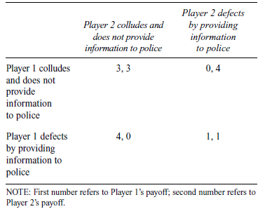
In this payoff bimatrix, the first number in each outcome indicates Player 1’s payoff should the corresponding outcome occur, and the second number indicates Player 2’s payoff in the corresponding outcome. For example, if both players collude, then every player will receive a payoff of 3. If both players defect, then each will receive a payoff of 1. The goal of every player in the game is to achieve the highest payoff by choosing one of two actions, given the action played by the other player. The payoffs can be ranked in order of desirability from 0 (least desirable) to 4 (most desirable). Desirability reflects the severity of the sentence. A payoff of corresponds to a more severe sentence than a payoff of 4. We can illustrate that in this prisoners’ dilemma, only the outcome in which both players choose to defect is a Nash equilibrium. Suppose Player 2 chooses to defect; if Player 1 chooses to defect too, Player 1’s payoff will be 1, which is higher than Player 1’s payoff of 0 if Player 1 chooses to collude. Applying the same argument to Player 2’s strategic thinking implies that Player 2 should choose to defect when Player 1 defects. In the prisoners’ dilemma, regardless of which strategy the other player chooses, it is always best to defect. More specifically, when Player 2 chooses to collude, Player 1 will receive a payoff of 4 by defecting, which is higher than his or her payoff of 3 by colluding. When Player 2 chooses to defect, Player 1 will receive a payoff of 1 by defecting as well, which is also higher than his or her payoff of 0 by colluding. In this case, defection is called a dominant strategy, and collusion is a dominated strategy. The best outcome for the two players is when they collude. However, collusion requires that both players choose dominated strategies.

In the Cournot model, between collusion and Cournot equilibrium outcomes, firms face a situation similar to the two suspects in a prisoners’ dilemma game. Although firms have higher profits together, it is not an equilibrium outcome, because every firm has an incentive to produce more than the amount agreed to. We will discuss how this collusive outcome may arise as an equilibrium outcome when firms interact repeatedly over time.

Bertrand Competition

The term Bertrand competition refers to the strategic situation when all the firms choose what prices they would like to charge for their products. When firms’ products are homogenous, consumers will purchase from the firms that charge the lowest price. Bertrand competition is also a standard strategic form game. However, the strategic situation faced by each firm is different from that in the Cournot competition. Because only the firms that set the lowest price are able to make a sale, a firm’s incentive in Bertrand competition is to cut the price of its product as long as it is still able to make profit. Applying this logic, every firm in the market will continue to slash its prices until there is no profit to make. When all the firms have a common constant marginal cost and no fixed cost, they will set the price at the constant marginal cost, which is also the constant average cost in this simple setting. If all firms set their prices at the average cost and one firm sets its price lower, this firm will make a loss. On the other hand, if a firm sets its price higher than the average cost, this firm will not make any positive sale, and hence, it has zero profit. Therefore, a firm does not have a profitable deviation when the other firms set their prices at the average cost of production. This equilibrium outcome in which all the firms choose the price at the average cost and every firm has zero profit is referred to as the Bertrand equilibrium.

Dynamic Oligopoly Models and Backward Induction

In a dynamic environment, the strategic interactions among firms are more complicated than in a static environment. A dynamic strategic interaction generally concerns an environment that involves sequential decision making by the agents. In a dynamic model, it is necessary to be more specific about when an agent chooses an action, what actions this agent can choose, and more importantly, what this agent knows at the time a choice of action is made. Because of this new element in dynamic strategy interaction, we must make the distinctions between actions and strategies more explicit. We first review how to model a dynamic game, as well as some widely used equilibrium concepts. Then we discuss a number of different dynamic oligopoly models to illustrate how economic agents interact in those dynamic settings.

Extensive Form Games

Researchers model dynamic strategic interactions using extensive form games. Extensive form games provide all the necessary elements, including the agents or the players of the game, the timing of each player’s choice of action, which actions each player may choose, what each player knows when choosing an action, and what each player cares about. Unlike in a strategic form game, the information available to a player when choosing an action is new in a dynamic game. As in static strategic problems, a player will choose an action based on the information available. One common way to summarize information available to a player is to introduce the history of past events up to the point at which the player chooses an action. In a dynamic game, every player needs to make a plan about which action to take after each possible event. A complete plan of action for a player, including one available action after every relevant event, is the player’s strategy. In other words, a strategy of a player in a dynamic game is a contingent plan of actions, a plan contingent on the histories available to the player. In a static game situation, there are no different stages of information, so the concept of strategies is the same as that of actions.

As in a static game, any list of strategies (or a strategy profile of one strategy by each player) will induce a complete path of plays, which can be considered as an outcome of the game. When choosing which strategy to play, a player evaluates strategies based on the outcomes that the strategies induce, given the strategies adopted by the other players.

Depending on how well a player knows what has happened, a dynamic game can have either perfect information or imperfect information. Perfect information refers to dynamic strategic situations in which every player knows exactly what has happened, including the actions taken by the players in the past. Many dynamic games in real life have perfect information, such as the game of chess, in which every player technically observes all the past steps. The formulation of extensive form games, however, does not exclude the possibility of some players choosing actions simultaneously, in which case the information structure is imperfect. Technically, we can collect the set of players, players’ strategies, and their payoffs to form a strategic form representation of a dynamic game. However, a strategic form representation of a dynamic game loses its dynamic information structure.

Nash Equilibrium and Subgame Perfect Nash Equilibrium

We can represent any dynamic game with a strategic form game. Any Nash equilibrium in the strategic form representation of a dynamic game is also a Nash equilibrium in the dynamic game. Because strategic representation of a dynamic game loses its information on dynamic structure of the model, applying the concept of Nash equilibrium in a dynamic game has been criticized because Nash equilibrium may involve some unreasonable behaviors, referred to as noncredible threats. Noncredible threats are the actions that are not one of the best responses given the history and what players will play in the future. Noncredible threats can be part of a Nash equilibrium strategy profile when they occur after histories that are unreachable for the given strategy profile, and hence, they are irrelevant to players’ payoffs. However, if those histories were reached, noncredible threats would not be carried out because they are not the best response given how the rest of the game will be played.

Applying the concept of Nash equilibrium in dynamic games oversimplifies the strategic reasoning. In a dynamic game, when any player chooses an action, this player should choose the best action available given the history and how the rest of the game ought to be played when the same reasoning is applied. In dynamic games with a finite horizon, this line of reasoning leads to the method known as backward induction. Backward induction analyzes the last stage of the game first. In games with perfect information, the problem in the last stage of the game is a simple decision problem; the active player simply chooses one of best available actions during the last stage of the game, given how the game has been played. Next, we analyze players’ strategic rationale in the second-to-last stage of the game, given how the game has been played and how the game will be played in the last stage of the game.

The problem faced by the active player in the second-to-last stage of the game is a well-defined decision problem induced by what will happen in the last stage of the game after every action of the players in the second-to-last stage. Accordingly, the active player will choose the best action induced by what will happen during the last stage. After identifying what will happen in the last two stages of the game, we then analyze the third-to-last stage and so on, and eventually we will solve a subgame perfect Nash equilibrium of the model. Backward induction eliminates noncredible threats so that any strategy profile resulting from backward induction does not suffer the criticism we discussed for applying the concept of Nash equilibrium in a dynamic game. In a dynamic game of perfect information, strategy profiles resulting from backward induction form a special class of Nash equilibria known as subgame perfect Nash equilibria.

There may not be well-defined stages in a dynamic game with imperfect information, so we cannot directly apply the backward induction technique used for games with perfect information. Instead, researchers first identify all situations in which the rest of the game can be viewed as a dynamic game itself. These situations are called the subgames of the underlying dynamic game. In fact, each stage of a dynamic game with perfect information is a subgame. After identifying all the subgames, we first derive Nash equilibrium outcomes in every subgame that does not include any other subgame—the class of smallest subgames. We then analyze subgames that contain only these smallest subgames, and the Nash equilibria that induce a Nash equilibrium in each of the smallest subgames it contains. Repeating this process leads to a Nash equilibrium of the entire game that induces a Nash equilibrium in any subgame. Accordingly, such a Nash equilibrium is subgame perfect Nash equilibrium. The concept of the subgame perfect Nash equilibrium is a widely adopted refinement of Nash equilibrium in economic research because of its simplicity. Many other refinements of the Nash equilibrium concept have been introduced and studied. The References: section provides some useful sources on the details of equilibrium refinements in extensive form games.

Stackelberg Model

The Stackelberg model refers to situations in which firms in oligopoly markets compete in their output, but firms do not all make their decisions at the same time. Naturally, the underlying strategic situation is a dynamic game. For simplicity, we discuss the Stackelberg model with two firms. One firm, called the quantity leader, chooses and commits to how much to produce. The other firm, called the quantity follower, first observes the amount of output by the quantity leader and then decides how much it will produce. In this subsection, we focus on this simple Stackelberg model and illustrate how various concepts and ideas for dynamic games are applied.

The Stackelberg model is a two-stage dynamic game with perfect information. To the quantity leader, there is a unique history when it makes a decision on how much to produce. Because the quantity follower observes how much the quantity leader has chosen to produce, each output level chosen by the leader is a history to the follower when it makes its decision about how much to produce. This difference sets the Stackelberg model apart from the Cournot model.

To apply the backward induction technique to find the subgame perfect Nash equilibrium in this Stackelberg model, first consider the second stage of the model in which the quantity leader has already committed to its output level. The strategic problem faced by the quantity follower simplifies to an ordinary monopoly problem with the residual demand, which is the difference between market demand and the amount of output committed to by the quantity leader. Applying exactly the same argument as in the Cournot oligopoly model, we can find the quantity follower’s best response to the amount of output by the quantity leader. The follower’s best response naturally varies with respect to the quantity leader’s output level and can be considered as the Nash equilibrium outcome in the subgame induced by the output quantity committed by the quantity leader.

When the quantity leader decides how much output to produce during the first stage of this Stackelberg model, it should able to anticipate how the quantity follower will respond. Taking the best response of the quantity follower into account, the problem faced by the quantity leader reduces to a decision problem because the amount of output by the quantity follower is uniquely determined by how much the quantity leader produces, and hence, the profit of the quantity leader is also uniquely determined by its output level. Any solution to this induced profit optimization problem for the quantity leader’s strategy is a subgame perfect Nash equilibrium of the Stackelberg model. The best response correspondence of the quantity follower is its equilibrium strategy because its best response specifies what the quantity follower should do in all possible subgames in the second stage of the model. The response of the quantity follower to the equilibrium strategy (quantity) of the quantity leader is what would happen in this subgame perfect Nash equilibrium, which is the equilibrium outcome. All other subgames in the second stage will be not reached, according to the equilibrium strategy of the quantity leader.

Repeated Strategic Interaction

In many economic and other strategic problems, players often interact repeatedly over many time periods. Because the strategic situation during each time period is the same, a repeated game model provides a relatively simple framework to study players’ long-term strategic behavior. People change their behavior when they consider the future as well as their immediate well-being. A well-known phenomenon in repeated interaction is the folk theorem; repeated interaction introduces many new equilibrium outcomes.

To illustrate how repeated interaction differs from its static counterpart, we revisit the Cournot model with two firms. Recall that the collusive outcome is not a Nash equilibrium in the static environment, even though both firms have higher profits than in the static Cournot-Nash equilibrium. Collusion cannot be sustained in equilibrium in the static Cournot model because every firm has an incentive to produce more. Nevertheless, when both firms value their future highly enough, collusion is possible when it is highly likely that the two firms will be involved in the

same Cournot competition in the future. Collusion can be sustained in a repeated Cournot model by a class of simple strategies known as grim trigger strategies. A grim trigger strategy profile calls for each firm to collude at the beginning of the repeated game and to continue to collude as long as both firms have colluded in the past, and as soon as either or both firms deviate, both firms will choose their Cournot-Nash equilibrium strategies forever. Any deviation from collusion triggers the Cournot-Nash equilibrium in the future, which serves as a punishment to the deviating firm. First observe that if a cartel breaks down, it is in each firm’s best interest to follow its Cournot-Nash equilibrium strategy. Now the question is what incentive each firm has to continue to collude if they have colluded in the past. Consider the following two possibilities: If a firm deviates away from the collusion outcome, its profit in the current period will be higher. However, such a deviation will trigger the static Cournot-Nash equilibrium forever. On the other hand, if it does not deviate, collusion will continue. Applying the same reasoning in every period, each firm is facing two sequences of profits when deciding whether to continue to collude: collusion forever or a higher profit in the current period followed by a lower profit from Cournot-Nash equilibrium forever. When it is highly likely that the two firms will be involved in the same situation again and again, and when every firm values the future highly enough, a firm will find it beneficial to forgo short-term gain in exchange for collusion in the future. Here we discuss only one particular subgame: perfect Nash equilibrium outcome in the infinitely repeated Cournot model. As matter of fact, all outcomes in which every firm has a profit may arise as an equilibrium outcome in the infinitely repeated Cournot model. This result is known as the folk theorem.

Conclusion

In this research paper, we took competition among oligopoly firms as a background to discuss a number of key concepts and model ideas in analyzing strategic interactions. We first considered how a perfectly competitive firm, and then a monopolistic firm, behaves, to pave the road for oligopoly problems. The key message is that firms make decisions in response to any change in the economic environment. In the rest of this research paper, we focused on oligopoly markets and analyzed how firms compete in various markets. We started with the Cournot model, in which firms compete in their outputs and make decisions simultaneously. This problem was formalized as a strategic game, and we applied the concept of Nash equilibrium to this model. Borrowing the idea of individual incentives, we have argued the collusive outcome in the Cournot model is not an equilibrium. We also discussed the Bertrand model, in which firms choose their prices simultaneously. We then moved to dynamic strategic interactions. We reviewed the Stackelberg model as an extensive form game and the concept of a subgame perfect Nash equilibrium. Economics of strategy applies game theory in economics and in business. Here we provided only a brief overview of firms’ strategic behaviors. Because of its versatility, game theory has been applied in virtually all areas of economics research and studies.

Bibliography:

1. Aliprantis, C. D., & Charkrabarti, S. K. (2000). Games and decision making. New York: Oxford University Press.
2. Besanko, D., Dranove, D., Shanley, M., & Schaefer, S. (2009). Economics of strategy. Hoboken, NJ: Wiley.
3. Cabral, L. M. B. (2000). Introduction to industrial organization. Cambridge: MIT Press.
4. Dixit, A. K., & Nalebuff, B. J. (1991). Think strategically: The competitive edge in business, politics, and everyday life. New York: W. W. Norton.
5. Dixit, A. K., & Skeath, S. (1999). Games of strategy. New York: W. W. Norton.
6. Friedman, J. (1989). Oligopoly theory. New York: Cambridge University Press.
7. Mendelson, E. (2004). Introducing game theory and its applications. New York: Chapman & Hall/CRC.
8. Osborne, M. J. (2004). An introduction to game theory. New York: Oxford University Press.
9. Osborne, M. J., & Rubinstein, A. (1994). A course in game theory. Cambridge: MIT Press.
10. Rasmusen, E. (2007). Games and information: An introduction to game theory (4th ed.). Malden, MA: Blackwell.
11. Shy, O. (1996). Industrial organization, theory and applications. Cambridge: MIT Press.