Fiscal Policy Research Paper

This research paper looks at the impact of government’s spending and tax policies, discussing the ways in which it can affect, and has affected, the economy. It also presents various arguments for greater reliance on fiscal policy to increase employment, as well as discusses the problems that increased government deficits may impose on future generations.

Federal Government Spending

Economists categorize government spending in two types. First, there is government purchases of goods and services. Government purchases of food, military goods, and other goods needed for consumption purchases, as well as purchases of investment goods, such as buildings and the building of bridges, are included. On the other hand, the government also spends on social insurance programs, such as Food Stamps and Medicare, which are primarily transfers of income from taxpayers to needy citizens. These are referred to as transfer payments.

Federal, state, and local governments all purchase goods and services and have the potential to affect economic activity. According to the 2008 Economic Report of the President, over the past 46 years, total government spending on goods and services, as well as federal spending by itself, has fallen as a percentage of GDP while state and local spending has increased as a percentage of GDP. Total government spending was approximately 19.1% of GDP in 2007: Federal spending was 7.1% of GDP while state and local spending was 12.2%. This compares with total government spending of 21.2% of GDP in 1960, when federal spending was 12.2% of GDP and state and local spending was 9.0%.

According to Alan Auerbach (2007), since 1962 there have been substantial changes in the components of government spending. He highlights the decrease in defense spending over this time with the notable exceptions of the first half of the Reagan administration and in the post-9/11 era. However, as Auerbach explains, “entitlement spending has more than doubled as a share of GDP since the early 1960s, absorbing the ‘peace dividends’ provided by the conclusions of the Vietnam and Cold Wars” (p. 215).

The Congressional Budget Office (2009) provides more insight into total government spending by dividing federal government spending into discretionary spending, mandatory spending net of any offsetting receipts, and net interest. Figure 1 below shows how federal spending as a percentage of GDP has changed over time from 1962 to 2007. Discretionary spending has fallen over time, mandatory spending has risen, and net interest has varied.

Figure 1 Components of Federal Spending SOURCE: Congressional Budget Office (2009)

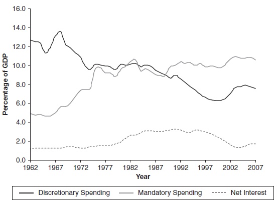
Discretionary spending consists of items on which Congress chooses to spend, such as defense and non-defense spending, while mandatory spending consists of programs where spending levels are already determined as a matter of law, such as spending on Social Security, Medicare and Medicaid, and other income, retirement, and disability programs, including unemployment compensation, Supplemental Security Income, and Food Stamps, among others. Figure 2 shows the changing composition of mandatory spending over time. The major changes in the percentage of the components of mandatory spending as a percentage of GDP occur in both Social Security and Medicare. As the baby boomers age, these components promise to become even larger components of mandatory spending.

Figure 2 Components of Mandatory Spending

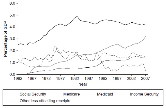
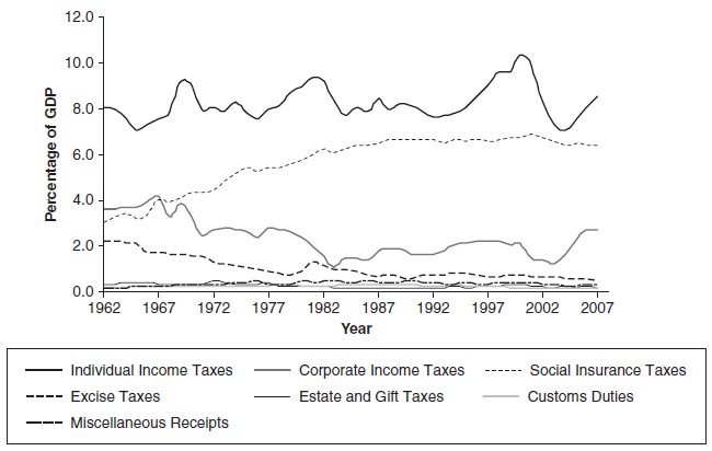
Figure 3 Components of Tax Revenue SOURCE: Congressional Budget Office (2009)

Federal Tax Revenue

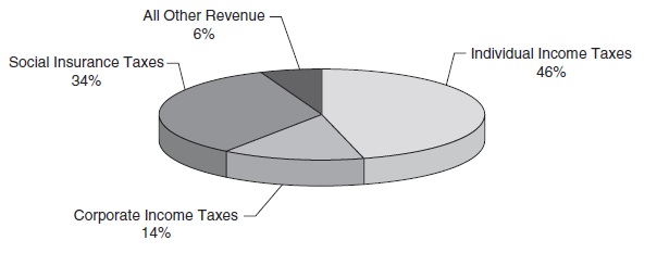
The federal government has several tax revenue streams, including individual income taxes, corporate income taxes, social insurance taxes (to fund programs intended to protect households from economic hardship), excise taxes (taxes on specific goods such as cigarettes), estate and gift taxes, custom duties, and other income streams. Figure 3 shows that individual income taxes are the most important source of tax revenue, followed by the recently more important social insurance taxes. The third most important source is excise taxes, with corporate income taxes, estate and gift taxes, and custom duties representing a small percentage of GDP. From another perspective, Figure 4 shows the sources of federal tax revenue in 2007. This figure again illustrates that 14% individual income taxes plus social insurance taxes represent almost 80% of all federal tax revenue.

Figure 4 Components of Federal Tax Revenue SOURCE: Congressional Budget Office (2009)

Personal income taxes in the United States are progressive, meaning that individuals with higher incomes pay a higher percentage of their income in taxes. In 2008, there were six different tax brackets with individuals paying a higher percentage of their income in taxes as their income rose. Although the income brackets change depending on whether the taxpayer is single, head of household, or married, the rates were 10%, 15%, 25%, 28%, 33%, and 35%. A report by the Congressional Budget Office to the Chair of the Finance Committee of the U.S. Senate in 2008 found that the tax system is indeed progressive in practice. The Congressional Budget Office reported that with regard to all federal taxes (not just income taxes), those individuals in the first income quintile (those whose income are among the lowest 20% in the country) pay an effective tax rate of 4.3% of income, those in the second quintile pay 14.2%, in the third pay 14.2%, and in the fourth pay 17.4%, while those whose incomes are among the 81% to 90% pay 20.3%, 91% to 95% pay 22.4%, 96% to 99% pay 25.7%, and those in the top 1% pay 31.5%.

Although it is difficult to compare tax burdens internationally, Forbes (Anderson, 2006) attempted to measure a Tax Misery & Reform Index that presents an international comparison of top marginal rates of taxation. The Misery scores are the sum of personal income taxes, corporate income taxes, wealth taxes, employer social security taxes, employee social security taxes, and VAT/sales taxes. From this analysis, it does not appear that Americans are particularly heavily tax burdened. Allowing for some differences within countries due to property and sales taxes, China and the original European Union-15 nations have the highest levels of tax misery, with index values ranging from 121.0 to 166.8, while the United States has an index value between 115.7 in New York and 94.6 in Texas.

Automatic Stabilizers

Fiscal policy also provides some automatic stabilization for the economy during the business cycle. For example, government spending on unemployment compensation, Supplemental Security Income, and Food Stamps will decrease (increase) during an expansion (recession), while personal income taxes will decrease (increase) during a recession (expansion). The decrease in taxes is also more than a proportional decrease. Because the personal income tax system is progressive (i.e., individuals pay a higher proportion of their income as the income rises), it may be that the decrease in income lowers not only the total amount of taxes paid but also the proportion of income paid in taxes. So as personal income falls (rises) during a recession (expansion), fiscal policy acts as an automatic stabilizer for income by increasing (decreasing) social insurance spending and lowering (raising) taxes, thereby helping to maintain a household’s income when the economy is in recession (expansion).

Social Security and Medicare

There is a great concern that government spending on Social Security and Medicare may soon overwhelm the budget and lead to larger and larger government deficits. According to Rudolph Penner and C. Eugene Steuerle (2007), “Discretionary programs now constitute less than 40 percent of spending, whereas they were almost 70 percent of spending in 1982” (p. 1). They also explain that although today about half of federal spending goes to benefit people aged 65 and over through the Social Security, Medicare, and Medicaid programs, they warn that by the year 2030, these “programs are expected to absorb between 5 and 9 percent more of gross domestic product than they did in 2006.” This is due to the increase in life expectancy and the improvement in health care. Adding to the problem is the fact that birthrates fell rapidly in the 1960s and remain low. As Penner and Steuerle explain, today’s labor force, and with it the number of taxpayers, is now growing slowly, but that growth is expected to decelerate in the future.

State and Local Government Spending and Tax Revenue

Although state and local governments may have individual income taxes, the primary ways in which they raise tax revenue is through property and sales taxes. According to the U.S. Census Bureau, in 2005 and 2006, almost 65% of all state and local tax revenue in the United States was in the form of property and sales taxes. Education, the largest single source of expenditure for state and local governments, is approximately 30% of total expenditure. It is followed by programs for social insurance and income maintenance at 22% of total expenditure and utility expenditure at 13.5%.

Theory

Macroeconomics is a relatively new branch of economics. Although classical economists had a framework for looking at the macroeconomy, they believed that any unemployment problem would be quickly resolved and that the economy would usually function at full-employment. They argued that production was a part of the consumption process. In other words, we produce goods and services because we want to sell them for money to buy what we want to consume. If we produced too many of some types of goods and services, the prices of those goods and services would fall, and we would no longer be able to buy the goods we wanted to consume. As a consequence, we would change what we were producing, and employment would rise in the production of the higher value goods. In the view of the classical economists, the economy would tend toward full employment, and there could not be any sustained unemployment.

It was with the Great Depression and the publication of John Maynard Keynes’s General Theory of Employment, Interest and Money that economists began to understand that there may be a role for government to play in influencing the level of output, employment, and prices. Keynes asserted that rather than supply creating demand, it was demand that creates supply, and therefore there could be a persistent oversupply of goods. There was no reason that the economy would tend toward full employment, and unemployment could be severe and persistent. Keynes argued that this was what was happening during the Depression. He also argued that the government could alleviate the unemployment by increasing demand through either increases in government spending or decreases in taxes.

Equilibrium Output and Equilibrium Income

National output (GDP) is determined by identifying the spending in the economy by the major players: households, firms, and government. Goods bought by households are defined as consumption (C), goods bought by firms as private investment (I), and goods bought by the government as government spending (G). If the economy does not engage in international trade, total demand equals consumption plus private investment plus government spending (i.e., C +1 + G). The economy will be in equilibrium when what is produced is exactly equal to what is demanded, or

Y = C + I + G,

where Y is total output produced. In this case, equilibrium output also represents equilibrium expenditure in the economy. Further, if mechanically expenditure must equal income, then Y also represents equilibrium national income.

If the economy is allowed to trade, some of the consumption, private investment, and government spending may be on goods that are not produced in the country; they may be on imports (IM). If this is the case, then these imports do not represent demand for goods produced in this country. However, it may be that foreigners will demand some goods that will be produced in this country; these are our exports (X). In an open economy, equilibrium will be achieved when domestic production equals the demand for domestic goods and services, or

Y = C + I + G + (X- IM).

There is no reason why domestic production should equal the domestic demand for goods and services at full employment. Full employment exists when workers who are willing and able to work at the going wage rate can find employment. It may be that the domestic production equals the demand for goods and services at a level of output that is less than full employment; if this is the case, the economy is in recession. Changes in government spending and taxes can help bring the economy to full employment. If an economy is in recession, the government can either

increase government spending or decrease taxes (if personal taxes decrease, consumption will increase), increasing domestic demand for goods and services. Production and employment will increase. If there is inflation in the economy, the government can either reduce its spending or raise taxes, reducing domestic demand for goods and services, thereby reducing inflationary pressure. When the government uses changes in government spending or taxes to affect economic activity, it is said that the government is using discretionary fiscal policy.

The Multiplier

According to Keynesian theory, the effect of a change in government spending or a change in consumption spending due to the change in taxes on equilibrium income will be larger than the initial change in spending. There will be a multiplied effect on output due to the initial change in spending because consumption spending itself is a function of disposable income (i.e., national income less taxes). The Keynesian view of consumption is that it is a function of disposable income. As disposable income increases, there will be a propensity to spend part of that increase and to save part of it. Given an additional dollar in disposable income, households will be likely to spend a certain percentage and to save a certain percentage. The percentage that it is likely to be spent is known as the marginal propensity to consume (mpc), while the percentage that it is likely to be saved is known as the marginal propensity to save (mps). The mpc plus the mps must equal 1.

Government Spending Multiplier

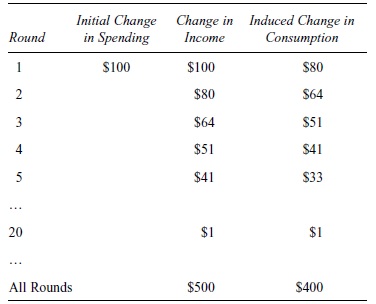
An example can illustrate how a change in government spending can have a multiplied effect on national income. Table 1 shows the changes in spending and income in this example. Suppose an economy were in equilibrium at a level of output less than full employment and the government increased its spending by $100 billion. Assuming that taxes are not a function of income but are a fixed amount per person, any increase in income will also increase disposable income by that amount. However, if the marginal propensity to consume in this economy is 80%, then the initial increase in income of $100 billion will also induce an increase in consumption spending of $80 billion. This induced increase in consumption spending also raises disposable income by $80 billion, leading to a further increase in consumption spending of $64 billion, and so on. The initial increase in spending (whether government spending or consumption spending due to a change in taxes) induces various rounds of consumption spending with each round spending (and income increasing) less and less. As Table 1 illustrates, if the mpc equals 80% and there is an initial increase in spending of $100 billion, this will induce a total increase in consumption spending of $400 billion and will ultimately increase equilibrium income by $500 billion. In this example, the multiplier is 5; with a mpc of 80%, any initial change in spending will increase equilibrium income by 5 times the initial change in spending. The value of the multiplier is

Multiplier = 1/(1 – mpc).

Table 1   The Government Spending Multiplier

The Tax Multiplier

The government could also have a positive effect on equilibrium national income by lowering taxes by $100 billion, but the effect on the increase in national income will be smaller. The value of the tax multiplier is smaller than the value of the spending multiplier. Table 2 illustrates this example. If the government lowers taxes by $100 billion, disposable income will rise by $100 billion. Given the mpc of 80%, this will result in an initial increase consumption spending of $80 billion and an increase in saving of $20 billion. In contrast to the preceding example, when government spending increased by $100 billion, it is the $80 billion increase in consumption spending that starts the multiplier effect. Ultimately, the $100 billion tax cut raises equilibrium national income by $400 billion. The tax multiplier is only 4; any decrease in taxes will increase equilibrium national income by 4 times the decrease in taxes. The value of the tax multiplier is

Multiplier = -mpc/(1 – mpc).

It is negative because a decrease in taxes will increase equilibrium national income and vice versa.

Proportional Taxes

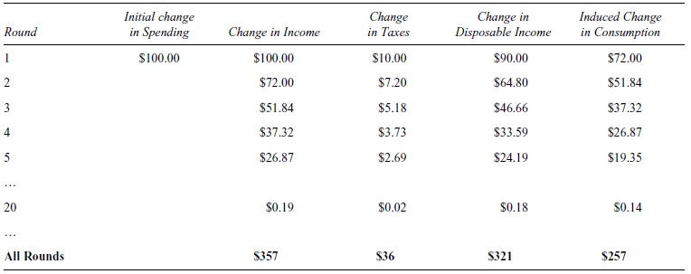
Relaxing the assumption that taxes are a fixed amount per person and introducing a proportional tax system (i.e., taxes are a function of income), the size of the multiplier decreases, but a change in government spending will still have a multiplied effect on equilibrium output. Continuing with the preceding example, one can determine the change in equilibrium income if the government increases its spending by $100 billion when the mpc is 80% and taxes are 10% of income. Because taxes are a function of income, disposable income equals national income minus taxes. In this case, as the government increases its spending by $100 billion, income rises by $100 billion, but now households will have to pay 10% of the increase in income in taxes leaving an increase in disposable income of only $90 billion. With an mpc of 80%, this will induce an increase in consumption spending of $72 billion. Table 3 shows the rounds of spending and income when a 10% proportional tax is imposed. The total change in equilibrium income is $357 billion (or approximately $36 billion in taxes and $321 billion in disposable income) with an induced change in consumption of $257 billion. With the introduction of a 10% tax rate, the value of the multiplier fell to 3.57 from 5. With a proportional tax, the value of the multiplier can be calculated as

Multiplier = 1/(1 – mpc + t*mpc),

where t is the tax rate.

Table 2   The Tax Multiplier

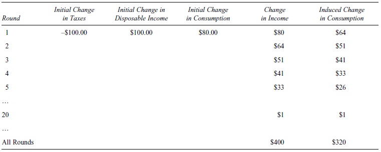
Table 3   The Proportional Tax Multiplier

This also explains why a proportional tax system is an automatic stabilizer for the economy. The introduction of the proportional tax system lowered the value of the multiplier. Anytime there is an exogenous change in any type of spending (i.e., consumption, private investment, or government spending), the change in equilibrium income will be smaller with proportional taxes than without, helping stabilize the economy.

“Fine-Tuning” the Economy

If the preceding example correctly represents how the economy actually works, then it appears rather easy for the government to use changes in government spending and changes in taxes to bring the economy to full employment. However, this is not the case. If the government could immediately (a) recognize that the economy is in recession, (b) agree to do something about the problem, (c) implement the program, and (d) get households and firms to respond to the plan, it might work. Unfortunately, each of these four steps takes time. The recognition, decision, implementation, and response lags take away valuable time during which the economy does not remain stagnant. It may be that by the time households respond to the plan, the economy will move from being in a recession. The policy taken to combat the recession will now be pointless or will create new problems for the economy. For this reason, fiscal policy is not used to “fine-tune” the economy—that is, keep the economy at full employment—but to combat persistent and significant macroeconomic imbalances.

Temporary Versus Permanent Fiscal Policy Measures

Another problem when using fiscal policy to combat either a recession or inflationary pressure is that the government may want to make the policies temporary so that when the economy recovers, the discretionary policy measures do not create any unintended problems. Unfortunately, if a fiscal policy action is known to be temporary, it may not be effective. According to the permanent income hypothesis, first asserted by Milton Friedman (1957), consumers base their consumption spending on what they view as their permanent income. Because changes in income that households do not see as permanent will not lead to changes in consumption spending, temporary fiscal policy measures may have very small multipliers. A classic example of this problem is the Revenue and Expenditure Control Act of 1968, which created a temporary tax surcharge to help alleviate inflationary pressures in the economy. However, households did not see the increased tax as permanent, and it did little to lower expenditures or inflationary pressure. As Alan Blinder and Robert Solow (1974) explain, “Prices rose faster after its passage than before” (p. 10).

Bias Toward Expansionary Fiscal Policy

The government can use expansionary fiscal policy, an increase in government spending or a reduction in taxes, to increase equilibrium income and contractionary fiscal policy, a decrease in government spending and increase in taxes, to reduce equilibrium income and inflationary pressures. With the exception of worrying about any government deficits that may result, expansionary fiscal policy is a much more attractive policy in popular political terms than contractionary fiscal policy. Although it is unlikely that everyone will agree about which spending should be increased or which taxes should be cut, voters will be more likely to vote for an elected official who does either. On the other hand, few elected officials would look forward to a reelection after either decreasing government spending or increasing taxes. William Nordhaus (1975) explained the possibility of the existence of a political business cycle in which an elected official would choose more contractionary fiscal policies at the beginning of one’s term but endorse more expansionary policies as the time for election draws new: “Moreover, with an incumbent’s term in office there is a predictable pattern of policy, starting with relative austerity in early years and ending with the potlatch right before elections” (p. 187).

Balanced Budget Rule

One of the dangers of expansionary fiscal policy is that it may increase the national debt. To finance a government budget deficit, the U.S. Treasury must borrow from either the public or the Federal Reserve by selling securities. A bias toward expansionary fiscal policy may lead to an ever-increasing national debt. To avoid this, there have been many calls for some type of balanced budget rule. However, whether the balanced budget rule is imposed through a constitutional amendment or some other mechanism, it would take away the ability of the government to use fiscal policy to counteract a recession and would also lead to greater instability in the economy (i.e., it will increase the value of the multiplier).

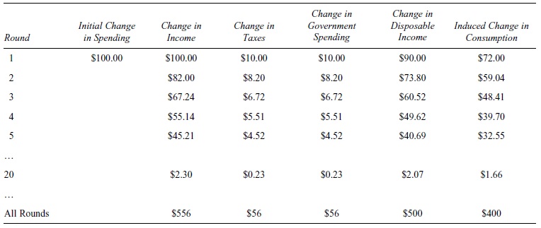
A balanced budget rule increases the value of the multiplier because it requires that when an exogenous decrease in spending lowers equilibrium income and threatens to bring the economy into recession, the government must reduce its own spending as tax revenues fall with income. Table 4 illustrates the particular example of a decrease of $100 billion in private investment spending, perhaps due to increased pessimism about the state of the economy among the business community. If the government is required to maintain a balanced budget, as private investment spending and income decreases, not only does this induce decreases in consumption spending, but tax revenues fall, which induce cuts in government spending to keep the government’s budget balanced. At each round, income decreases because of decreases in both consumption expenditures and government expenditures. On net, the decrease in private investment spending will decrease equilibrium income by $556 billion; the multiplier is 5.56. With proportional taxes and a balanced budget rule, the multiplier is

Multiplier =   1/[(1 – mpc)*(1 -t)].

Without a balance budget rule, this same $100 billion decrease in private investment would have decreased equilibrium income by only $357.

A major disadvantage of a balanced budget rule is the increase in the value of the multiplier. Anytime there is a major decrease (increase) in spending, not only can the government not use expansionary (contractionary) fiscal policy, but the resulting decrease in national income or inflationary pressure will be worse than if the government was not forced to respond to the change in spending.

Table 4   The Balanced Budget Multiplier

Full-Employment Budget Balance

Although the budget deficit worsens when the government uses expansionary fiscal policy and improves when it uses contractionary fiscal policy, the budget balance by itself may not be a good measure of whether the government is using expansionary fiscal policy. The budget deficit also changes with the business cycle. As an economy expands, tax revenues rise and government spending on social insurance programs falls; the government’s deficit gets smaller. This is true whether or not the government is concerned that the economy’s expansion may be excessive. So if the government’s deficit is getting smaller while the economy expands, it is impossible to determine whether the decrease is due to automatic stabilizers or to discretionary fiscal policy just by looking at the net change in the budget balance. The same is true if the economy is heading into a recession. In that case, there would be a worsening of the budget deficit whether or not the government engages in expansionary fiscal policy. However, it is possible to calculate what the government’s budget balance would be if the economy were at full employment. Also known as the cyclically adjusted budget balance, it adjusts the actual budget balance for any extra tax revenue the government would collect or social insurance payments it would save if the economy were not in a recession. With this control, if there is an increase in the full-employment budget balance, it must be because the government is engaging in contractionary fiscal policy while any decrease would indicate expansionary fiscal policy.

The Problem of Crowding Out

Using expansionary fiscal policy may have some unintended consequences that can decrease the value of the multiplier. When the government increases its spending or decreases taxes, its budget balance declines. The only way the government can finance a deficit is to sell U.S. Treasury securities and, depending on who buys the securities, the increased deficit may lead either to increased inflationary pressure or higher interest rates.

If the government finances the deficit by selling U.S. Treasury securities to the Federal Reserve, this will increase the money supply and potentially increase inflationary pressure. Increases in the money supply will lower interest rates, encourage interest-sensitive consumption and private investment spending, and, if the economy is close to full employment, lead to increases in the price level.

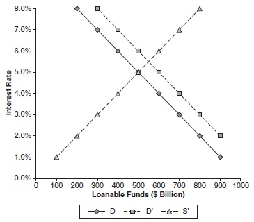
On the other hand, if the government finances the deficit by selling U.S. Treasury securities to the public, this will put upward pressure on interest rates. This can be seen in the loanble funds market in Figure 5. The demand for loanable funds comes from the borrowing needs of businesses and government, and is inversely related to the interest rate. Because each possible private investment project available has an expected rate of return, businesses will take on those projects for which the expected rate of return exceeds the interest rate. As the interest rate falls, more projects are profitable, leading to an increase in the quantity of loanable funds demanded. This assumes that the government deficit, that is, demand for loanable funds on the part of the government, is not related to the interest rate but is determined by the size of the deficit. The supply of loanable funds reflects the relationship between saving and the interest rate in the economy. As the interest rate increases, the reward for saving increases, and there is an increase in the quantity supplied of loanable funds. In the figure, D shows the demand for loanable funds before the expansionary fiscal policy, and D’ is the demand for loanable funds with the increased borrowing needs of $100 billion from the government. Prior to the government engaging in expansionary fiscal policy and increasing its demand for loanable funds, the equilibrium interest rate is 5% and the equilibrium level of loanable funds is $500 billion. After the government borrows $100 billion to cover its deficit, the equilibrium interest rate rises to 5.5% and the equilibrium level of loanable funds rises to $550 billion. Because the government’s share of loanable funds rose by $100 billion, but the total amount of loanable funds rose by only $50 billion, the increase in the interest rate must have decreased the quantity demanded of loanable funds by $50 billion. In other words, the increased borrowing needs of the government crowded out private investment.

Figure 5  The Market for Loanable Funds

Additionally, the increase in interest rates may affect the exchange rate leading to changes in the trade balance that further reduce the effectiveness of expansionary fiscal policy. As interest rates in the United States increase, both domestic residents and foreigners will want to buy U.S. assets. In the market for the U.S. dollar, this will increase the demand for dollars (foreigners wanting to buy U.S. assets first need to buy U.S. dollars) while decreasing the supply (Americans who may have bought foreign assets and consequently foreign currencies will not do so). Both factors will lead to an appreciation of the dollar and encourage an increase in U.S. imports of foreign goods and services while discouraging foreign purchases of U.S. exports. This decrease in expenditure on domestic goods and services will further limit the increase in equilibrium income in response to the expansionary fiscal policy.

It is even possible that there may be complete crowding out of private investments. Given the effects on the interest rate and the exchange rate, the increase in government spending might just provoke a decrease in spending on domestic goods and services that completely offsets any increase in national income.

Ricardian Equivalence

An alternative view of why expansionary fiscal policy may not increase national income is the Ricardian equivalence theorem. As Robert Barro (1992) explains it, the demand for goods by households is a function of the expected present value of taxes. Households determine how much to consume based on their net wealth position or the expected present value of income less the expected present value of taxes. Any increase in government spending or decrease in taxes financed through an increase in the deficit will only lead to an increase in expected future taxes equal to the same present value as the fiscal policy stimulus and will not lead to an increase in consumption spending. In Barro’s (1989) words, “Fiscal policy would affect aggregate consumer demand only if it altered the expected present value of taxes” (p. 39).

Empirical Evidence

Although the advocacy of fiscal policy to affect the economy began with John Maynard Keynes’s publication of The General Theory of Employment, Interest and Money, it was only when the government increased military spending for World War II that his theory was truly implemented. During the Great Depression, Franklin Roosevelt experimented with Keynesian theory when he implemented the New Deal. Although the programs of the New Deal were implemented prior to the publication of General Theory, its emphasis on increased government spending to stimulate the economy is exactly what Keynes was advocating.

After World War II, Keynesian economics and the beneficial effects of fiscal policy were definitely in vogue. Through the 1950s and 1960s, the economy behaved in a manner similar to the Keynesian model. The economy varied between times of low unemployment and high inflation and of high unemployment and low inflation. The Keynesian policy prescription was clear: Use expansionary fiscal policy to cure an unemployment problem and a contractionary one to cure inflation.

Emphasis on Monetary Policy

Unfortunately, in the 1970s, the rapid increase in the price of oil appeared to change the relationship between unemployment and inflation. During this time, the economy experienced stagflation, that is, the combination of both unemployment and inflation. The Keynesian model seemed to be failing to explain the economy, and fiscal policy did not seem to hold much potential to mitigate the problems. At the same time, increases in the size of the U.S. government deficit and national debt caused many to worry about the effects of further expansionary fiscal policy on future generations. According to John Taylor (2000), by the end of the 1970s,

discretionary countercyclical fiscal policy was no longer considered a serious policy option in the United States. As Laurence Seidman (2001) explains, “Whereas Congress enacted a major fiscal stimulus package to counter the 1975 recession, it did not even consider a serious package in the 1991 recession” (p. 18). The focus had shifted to the use of monetary policy. As Taylor (2000) writes, “Over the [1980s and 1990s], the Federal Reserve’s interest rate decisions have become more explicit, more systematic, and more reactive to change in both inflation and output” (p. 21). The economy performed well under this regime with only two relatively mild recessions, one in 1980 to 1982 and one in 1990 to 1991.

However, signs of the weakness of monetary policy became apparent when looking at the slump in the Japanese economy. After amazing postwar growth that propelled war-torn Japan to a major industrial nation, a real estate and stock market boom in the 1980s was followed by a crash in both markets and a period of relatively slow growth or recession since 1991. This period has also been characterized by very low interest rates as the Bank of Japan tried to stimulate the economy with expansionary monetary policy. Similar to our experience during the Great Depression, the Japanese economy had fallen into a liquidity trap. First described by Keynes, a liquidity trap is when interest rates are at or close to zero but the low interest rates do not spur interest-sensitive spending. Because an expansionary monetary policy affects the economy when an increase in the money supply lowers interest rates and encourages interest-sensitive spending, when interest rates are at or close to zero, there is little impact on the economy. As in the Great Depression with the impotence of traditional monetary policy, Japan turned to fiscal policy to help promote growth in the economy.

Economic and Financial Crisis of 2008

After a relatively long expansion and large increases in stock price during the late 1990s, the economy began to show signs of weakness in early 2000. What has been called the dot-com bubble, the large increase in the stock prices of technology stocks, burst in early 2000, and for most of 2001, the economy was in recession. The recession, along with the terrorist attacks of September 11, 2001, led the Federal Reserve to lower interest rates significantly. The Fed lowered the target federal funds rate 11 times in 2001 from a rate of 6.00% to 1.75%. The decrease in interest rates helped lead the economy out of recession in part by increasing the demand for new homes. Housing prices soared along with consumer spending in response to higher wealth and to lower interest rates. From the beginning of 2001 until housing prices peaked in mid-2006, according to the S&P/Case-Shiller Price Index, housing prices essentially doubled in 10 major metropolitan cities. However, once housing prices began to fall and the subprime mortgage crisis ensued, the economy began to slow and went into recession in December 2007. Although the Federal Reserve attempted to encourage consumption and private investment spending through further decreases in interest rates, by the end of 2008, the target rate for the federal funds rate was essentially zero, and the U.S. economy faced its own liquidity trap. Although the Federal Reserve continued to provide liquidity into the markets through various lending facilities and quantitative easing, policy makers began looking once again to fiscal policy to help the economy out of recession.

Size of the Multipliers

A major controversy about using fiscal policy concerns the size of the government spending and tax multipliers. As previously discussed, the multipliers depend on the magnitude of the marginal propensity to consume and the tax rate. However, it is not so simple to calculate the size of the multipliers in the real world. E. Cary Brown (1956) was one of the first to attempt to estimate the sizes of the multipliers by looking at the effectiveness of fiscal stimulus during the Great Depression. Using Brown’s work, Gauti Eggertsson (2006) measured the real spending (holding the budget deficit constant) multiplier to be 0.5 and the deficit spending (cutting taxes and accumulating debt while holding real government spending constant) multiplier as 2 during the 1930s.

More recent estimates on the values of the multiplier vary widely and are the topic of great debate within the economics profession. Olivier Blanchard and Roberto Perotti (2002) estimate that the value of the multipliers are close to 1. They explain, “While private consumption increases following spending shocks, private investment is crowded out to a considerable extent. Both exports and imports also fall.” On the other hand, Eggertsson (2006) finds that “each dollar of real government spending increases output by 3.37 dollars and each dollar of deficit spending increases output by 3.76 dollars. These multipliers are much bigger than have been found in the traditional Keynesian literature.” Christina Romer, President Obama’s Chair of the Council of Economic Advisors, and Jared Bernstein, chief economic advisor to Vice President Biden, arguing in support of the American Recovery and Reinvestment Plan, estimate the output effects of a permanent increase of government purchases of 1% of GDP to be 1.57% after 10 quarters, and of a permanent tax cut of 1% of GDP to be 0.99%.

Future Directions

A big challenge facing fiscal policy in the future is meeting the increasing costs of Social Security, Medicare, and Medicaid programs. Penner and Steurele (2007) estimated that between 2006 and 2010, the cost of these three programs would grow by $326 billion, while the growth in tax revenues is expected to be only $494 billion. As they explain, “The three programs will absorb two-thirds of all revenue growth, even though they still only constitute[d] about 40 percent of total spending in 2006” (p. 3). Barring a broad reform of these programs, Penner and Steurele argue that some type of “trigger” system for these benefits be constructed. For example, a trigger system would set a particular growth rate for these benefits when the economy is close to full employment and another during a recessionary period.

Seidman (2001) argues for improving existing automatic stabilizers. As he asks, “Why not automatically trigger a tax cut in a recession?” (p. 39). By this, Seidman means a tax cut in addition to the automatic fall in revenue due to our progressive tax structure. Such a trigger would not require any legislative action but therefore would occur much more quickly than under the current system.

Another important discussion concerns the highly political atmosphere in which fiscal policy is set. Having served on both the Council of Economic Advisors and the Board of Governors of the Federal Reserve System, Blinder (1997) describes his different experiences with the setting of fiscal and monetary policies. Whereas monetary policy is in the hands of the Federal Reserve, an agency relatively independent of politics, fiscal policy is the result of a highly political process. As Blinder explains, although a policy discussion begins with social welfare as its main goal, it often “turns to such cosmic questions as whether the chair of the relevant congressional subcommittee would support the policy, which interest groups would be for and against it, what that ‘message’ would be, and how that message would play in Peoria.” The Economist (“Fiscal Flexibility,” 1999) has called for serious consideration of an independent fiscal authority. Seidman (2001) proposed that members of such a group would be appointed in a similar manner as the members of the Federal Reserve. The budget would continue to be set by the president and Congress, and “the board would implement periodic adjustments in taxes and government spending relative to the budget enacted by Congress.”

Conclusion

Fiscal policy has been and continues to be an important stabilization policy of the government. This research paper reviews the theory of fiscal policy and how it has been used in the United States. It gives insight into some of the major debates surrounding fiscal policy and future directions for research. Although the efficacy of discretionary policy measures continues to be debated and there is concern about the growing expenditures for Social Security, Medicare, and Medicaid, government spending and taxes will continue to be an important component of the policy toolbox available to influence the economy.

Bibliography:

1. Anderson, J. (2006, May 22). Tax misery and reform index. Forbes. https://www.forbes.com/global/2006/0522/032.html
2. Auerbach, A. J. (2007). American fiscal policy in the post-war era: An interpretive history. In B. Eichengreen, D. Stiefel, & M. Landesmann (Eds.), The European economy in an American mirror (pp. 214-232). New York: Routledge.
3. Barro, R. J. (1989). The Ricardian approach to budget deficits. Journal of Economic Perspectives, 3(2), 37-54.
4. Bayoumi, T., & Sgherri, S. (2006, July). Mr. Ricardo’s great adventure: Estimating fiscal multipliers in a truly intertemporal model (IMF Working Paper). https://papers.ssrn.com/sol3/papers.cfm?abstract_id=920260
5. Blanchard, O., & Perotti, R. (2002). An empirical characterization of the dynamic effect of changes in government spending and taxes on output. Quarterly Journal of Economics, 117(4), 1329-1368.
6. Blinder, A. S. (1997). Is government too political? Foreign Affairs, 76(6), 115-126.
7. Blinder, A. S., & Solow, R. M. (1974). Analytical foundations of public policy. In S. Blinder, R. M. Solow, G. F. Break, & P. O. Steiner (Contributors), The economics of public finance (pp. 3-118). Washington, DC: Brookings Institution.
8. Brown, E. C. (1956). Fiscal policy in the ‘thirties: A reappraisal. American Economic Review, 46(3), 857-879.
9. Congressional Budget Office. (2008, December 23). Historical effective tax rates, 1979 to 2005: Supplement with additional data on sources of income and high-income households. https://www.cbo.gov/publication/20374?index=9884
10. Congressional Budget Office. (2009, January 7). Revenues, outlays, surpluses, deficits, and debt held by the public, 1968 to 2007. https://www.cbo.gov/data/budget-economic-data#2
11. Economic report of the president. Transmitted to the Congress February 2008, together with the annual report of the Council of Economic Advisers. (2008). Washington, DC: Government Printing Office. https://fraser.stlouisfed.org/files/docs/publications/ERP/2008/ERP_2008.pdf
12. Eggertsson, G. B. (2006). Fiscal multipliers and policy coordination (Federal Reserve Bank of New York Staff Reports No. 241).
13. Fiscal flexibility. (1999). The Economist, 353(8147), 80.
14. Friedman, M. (1957). A theory of the consumption function: A study by the National Bureau of Economic Research. Princeton, NJ: Princeton University Press.
15. Keynes, J. M. (1936). The general theory of employment, interest and money. New York: Harcourt, Brace.
16. Krugman, P. (1998). It’s baaack: Japan’s slump and the return of the liquidity trap (Brookings Papers on Economic Activity No. 29). https://www.brookings.edu/wp-content/uploads/1998/06/1998b_bpea_krugman_dominquez_rogoff.pdf
17. Micl,T. (2008). Rethinking fiscal policy. Challenge, 51(6), 91-104.
18. Nordhaus, W. D. (1975). The political business cycle. Review of Economic Studies, 42(2), 169-190.
19. Penner, R. G., & Steuerle, C. E. (2007, August 1). Stabilizing future fiscal policy: It’s time to pull the trigger. The Urban Institute. https://www.urban.org/research/publication/stabilizing-future-fiscal-policy
20. Romer, C., & Bernstein, J. (2009, January 9). The job impact of the American Recovery and Reinvestment Plan. https://www.economy.com/mark-zandi/documents/The_Job_Impact_of_the_American_Recovery_and_Reinvestment_Plan.pdf
21. Schultze, C. L. (1992). Is there a bias toward excess in U.S. government budgets or deficits? Journal of Economic Perspectives, 6(2), 25-43.
22. Seidman, L. (2001). Reviving fiscal policy. Challenge, 44(3), 1742.
23. Spencer, R. W., & Yohe, W. P. (1970, October). The “crowding out” of private expenditures by fiscal policy actions. Federal Reserve Bank of St. Louis Review, pp. 12-24.
24. Standard & Poor’s. (2009). Case-Shiller home price history. https://fred.stlouisfed.org/series/CSUSHPINSA
25. Taylor, J. B. (2000). Reassessing discretionary fiscal policy. Journal of Economic Perspectives, 14(3), 21-36.
26. U.S. Census Bureau. (2008, July 1). State and local government finances by level of government and by state: 2005-06. http://www.census.gov/govs/www/estimate06.html