Cost-Benefit Analysis Research Paper

1. Identify the relevant population of the project. For a cost-benefit analysis of a single individual or for a firm, this is not a problem. But in a societal cost-benefit analysis, we need to consider how to define society. A common approach is to consider the whole country as the relevant population. This is reasonable given that most public policies are financed at the national level. Another approach is to conduct a cost-benefit analysis specifying costs and benefits using different definitions of the relevant population—for example, including benefits and costs of a neighboring country in the analysis.
2. Specify all the relevant benefits and costs associated with the policy. The aim with a cost-benefit analysis is to include all relevant costs and benefits with a policy. Based on the definition of the population (Step 1), every aspect that individuals in this population count as a benefit or a cost should be included in the analysis. For some benefits and costs of a policy, this may be an easy task—for example, 2,000 hours of labor input are required next year to build a road. But there are also more difficult phases in this step of a cost-benefit analysis; some examples include (a) a new infrastructure investment may have ecological consequences that are difficult to estimate and (b) regulating speed limits in a major city may have beneficial health effects due to decreases in small hazardous particles. For the economist or analyst, this step often consists of asking the right questions and gathering the necessary information from the literature, professionals, or both.
3. Translate all the benefits and costs into a monetary metric. A cost-benefit analysis requires that the different consequences are expressed in an identical metric. For simplicity, we use a monetary metric ($ or €, etc.). Consider the example of an investment in a new road. The costs for the labor input can be valued by the wages (plus social fees, etc.), and the use of equipment may be estimated by the machine-hour cost. For benefits of, for example, increased road safety, decreased travel time, and decreased pollution level, there are no market prices to use; instead, weights and estimates are necessary to translate these benefits into a monetary metric. If this would not be possible with all relevant consequences, they should at least be included as qualitative terms in the evaluation. In the Valuation of Nonmarket Goods section, giving nonmarket goods a monetary estimate is discussed.
4. If benefits and costs arise at different times, convert them into present value using an appropriate social discount rate. Most people prefer a benefit today to a benefit in one year. There are several reasons for this, one being that no one knows for sure whether he or she will be alive in a year. Another reason may be that, over a longer time horizon, people expect their incomes to increase in the future. If an extra dollar has a larger utility benefit to a less rich individual, that individual would prefer to consume when he or she has less money (today) rather than when he or she has more (e.g., in 5 years). Also, from an opportunity-cost approach, $100 that is not consumed today can be invested in a bond, and in a year from now, it may be worth $105, implying higher consumption in one year. In a cost-benefit analysis, economists therefore (generally) do not treat benefits and costs that occur at different times as equal; rather, they translate all benefits and costs into a present value. Choosing an appropriate social discount rate is, however, a complicated task and will often have major effects on the results of the evaluation. In the Discounting section, this is discussed in more detail.
5. Compare the net present value of benefits and costs. When the present value of benefits (PVB) and costs (PVC) has been calculated, what remains is to calculate the net present value (NPV). The policy is said to increase social welfare if the net present value is positive—that is, PVB- PVC> 0. It is also common to express the comparison as the benefit-cost ratio—that is, PVB / PVC, which gives the relative return of the investment. If the ratio is greater than 1, the policy increases social welfare.
6. Perform a sensitivity analysis to see how uncertain the benefit-cost calculation may be and give a policy recommendation. A cost-benefit analysis will have several uncertainties regarding the outcome. It is most often not reasonable to show only one point estimate of the evaluation. There are often uncertainties regarding both parameter values (such as the monetary estimates of, e.g., increased safety or environmental pollution) and more technical issues, such as the economic lifetime of a new road, which is the period during which it retains its function. These uncertainties need to be explicitly modeled. The final step in a cost-benefit analysis is to give a policy recommendation based on the result of the evaluation as well as the uncertainties associated with the result.

What Do We Mean by Social Welfare?

The aim with a cost-benefit analysis is to evaluate the welfare effect of a policy. This requires a definition of what is meant by social welfare in an economic framework. The meaning of a welfare improvement is, in its most restricted view, formulated in the Pareto criterion. The Pareto criterion states that a policy that makes at least one individual better off without making any other individual worse off is a Pareto-efficient improvement and increases welfare. However, the Pareto criterion is generally useless as a definition for welfare improvements in a real-world application, because more or less all policies make at least someone worse off. It may also be criticized on ethical grounds; consider a vaccine that would save 1 million lives in sub-Saharan Africa but required a €1 tax on someone (a nonaltruistic individual) in Europe or the United States. According to the Pareto criterion, this policy could not be said to increase welfare, but this conclusion would violate the moral values of most individuals.

As a development to the Pareto criterion, the Kaldor-Hicks criterion was formulated, and it may be seen as the foundation of practical cost-benefit analysis. The Kaldor-Hicks criterion is less restrictive than the Pareto criterion and may be interpreted such that a policy is considered to increase welfare if the winners from a policy are made so much better off that they can fully (hypothetically) compensate the losers and still gain from the policy (potential Pareto improvement). This implies that every Pareto improvement is a Kaldor-Hicks improvement, but the reverse is not necessarily true. The compensation from the winners to the losers is a hypothetical test, and the compensation does not need to be enforced in reality (which distinguishes it from the Pareto criterion). In the example above, the vaccine to save 1 million lives would pass the Kaldor-Hicks criterion, if those who were saved would be hypothetically willing to compensate the European taxpayer with a payment of at least €1. Cost-benefit analysis is a test of the Kaldor-Hicks criterion, translating all the benefits and the costs into a monetary metric. The Kaldor-Hicks criterion also implies that we need to collect information only on aggregate benefits and costs of a policy; we do not need to bother ourselves determining which individuals are actually winning or losing from a policy.

Valuing Benefits and Costs

Performing a cost-benefit analysis of a policy requires that all benefits and costs of the policy be summed up in monetary terms. There are two principal ways of measuring the sum of benefits in a cost-benefit analysis: willingness to pay (WTP) and willingness to accept (WTA). Both WTP and WTA are meant to value how much a certain policy is worth to an individual in monetary terms. The WTP of a policy may be characterized as an individual’s maximum willingness to pay, such that he or she is indifferent to whether the policy is implemented— that is, if it is implemented, utility is the same after the policy as before the policy. The WTA of a policy may instead be characterized as the lowest monetary sum that an individual accepts instead of having the investment implemented—that is, utility is the same when receiving the money as it would have been if the investment had been implemented. WTP and WTA for a policy are expected to differ (WTP < WTA) because of the income effect. Robert D. Willig (1976) shows, using plausible assumptions, that WTP and WTA should not differ from each other by more than a few percentage points. But a lot of research has documented that WTP and WTA usually differ a lot for the same policy, with WTA being significantly higher than WTP. Several hypotheses have been put forward trying to explain this discrepancy, one frequent hypothesis being the existence of an endowment effect (Kahneman, Knetsch, & Thaler, 1990). An endowment effect states that individuals value a good significantly more once they own it, which would create a gap between WTP and WTA for an identical good. In several circumstances, it is often more problematic to estimate WTA for a good, especially in valuation of nonmarket goods, implying that it is more common to use the concept of WTP in cost-benefit analyses.

The cost of a certain policy is based on the opportunity cost concept—that is, the value of the best alternative option that the resources could be devoted to instead. The opportunity cost is derived based on companies’ marginal cost curve—that is, the cost that is associated with increasing output with one unit. This should not be equalized to accounting costs, which do not necessarily tell us the economic cost of an activity. As an example, going to a 2-year MBA program has some direct costs (accounting costs), such as tuition fees, books, and travel costs to attend lectures, but also indirect costs, such as the money that one could earn in a job if not attending the MBA program. The economic cost of an activity is the sum of direct and indirect costs.

Valuation of Market Goods

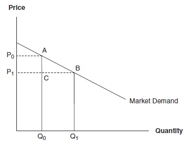
To estimate benefits and costs of a policy, the natural starting point is to examine whether market prices exist that may be used. If the market is characterized by perfect competition, or a reasonable approximation of perfect competition, and no external effects exist, the market price can give us information about the willingness to pay for a marginal change of a good. For example, if we need to use production factor X for a certain investment and our demand for X will not affect the market price, we can use the market price as a cost measure. The total cost of the production factor in the cost-benefit analysis is, then, the market price multiplied by the number of units used. However, if the policy will also affect the market equilibrium, we cannot simply use the market price in our analysis. Figure 1 shows the difference.

Initial market equilibrium is at price P0 and quantity Q0. Imagine that a new policy will lead to a decrease in the market price to P1, which increases quantity consumed to Q1. The total benefits of this policy include the increased consumer surplus for the original consumers (rectangular area P0P,AC) as well as the benefit of the new consumers (triangle area ABC). Hence, the total benefit may be represented by the area P0P,AB, which shows that when a policy has a nonmarginal effect on the market price, we cannot simply use the prepolicy market price in a cost-benefit analysis.

Figure 1.   Measuring Benefits and Costs for Nonmarginal Changes in Quantity

Other problems to note when using market data as information on prices in a cost-benefit analysis include market imperfections, such as tax distortions and externalities. The existence of taxes implies that there are several market prices, including or excluding taxes. An easy rule of thumb is to calculate prices including taxes, which implies that prices are expressed as consumer prices rather than producer prices. This implies that, for example, labor costs should be calculated as gross wages plus other social benefits or taxes that the consumer (or employer) has to pay. There is also another important effect of taxes that needs to be considered. Usually, cost-benefit analyses are performed for public projects, which often are paid for by taxes that lead to distortions in the economy. Distortions are created because not all activities are taxed, such as leisure. This implies that taxes on labor incomes change the relative prices between labor and leisure and lead to economic inefficiency. The distortion should normally be included in a cost-benefit analysis. As an example, in Swedish cost-benefit analysis, the recommendation is to include a distortion cost of 30% of direct costs (including taxes).

A final complicating note is that theoretically it may be that the correct benefit measure is the option price of a policy, which consists of the expected surplus (as outlined above) as well as the option value of a policy. Option value is the value that individuals are willing to pay, above the expected value of actually consuming the good, to have the option of consuming the good at some point in time (Weisbrod, 1964). For example, investing in a new national park includes the expected surplus of actually going to the park for the visitors. But it may also include a willingness to pay reflecting that the national park provides an option to go there, even if an individual will never actually go. In practical applications, it is common to exclude option value in the benefit calculations. There are several arguments for this; for example, it is difficult to measure and separate option values from other types of values or attitudes that may not be relevant, such as non-use values (non-use value refers to value an individual may place on, e.g., saving the rain forest in a specific region in South America, even if the individual knows that he or she will never go there—an intrinsic value). In addition to option value, sometimes it is also argued that a quasi-option value (sometimes referred to as real option) should be included in a project evaluation. The quasioption value refers to the willingness to pay to avoid an irreversible commitment to the project right now, given expectations of future growth in knowledge relevant to the consequences of the project. It is not particularly common to include quasi-option value in cost-benefit analyses.

Valuation of Nonmarket Goods

A common difficulty with a cost-benefit analysis is the fact that the policy to be evaluated includes a nonmarket good that is publicly provided. This implies that there are no market data to use. Examples of nonmarket goods that are common in cost-benefit analyses of public policy are values of safety, time, environmental goods, and pollution. Generally, there are two main approaches available for estimating monetary values of nonmarket goods: (1) revealed preference (RP) methods and (2) stated preference (SP) methods. RP methods use actual behavior and try to estimate implicit values of WTP or WTA. SP methods use surveys and experiments where individuals are asked to make hypothetical choices between different policy alternatives. Based on these choices, the researcher can estimate WTP or WTA.

Revealed Preference Method

Revealed preference techniques can be used to elicit willingness to pay when there is market information about behavior that at least indirectly includes the good that the analyst is interested in evaluating.

One revealed preference approach is hedonic pricing (Rosen, 1974). Imagine that we would like to estimate the willingness to pay to avoid traffic noise; we may be able look at the housing market in a city to accomplish this. The price of a house depends on many different characteristics: size, neighborhood, number of bedrooms and bathrooms, construction year, and so on. But another important determinant may be the level of noise—that is, a house located close to a heavily trafficked highway will generally be less expensive than an identical house located in a noise-free environment. The hedonic pricing approach uses this intuition and performs a regression analysis where the outcome is the market value of a house including several relevant characteristics as determinants of the house price (including the noise level, measured in decibels). The results from such a statistical analysis can in a second step tell us the impact of the noise level on the market price, holding other important factors constant. For example, Nils Soguel (1994) uses data on monthly rent for housing in the city of Neuchatel in Switzerland and included factors measuring the structure and condition of the building, several apartment-specific factors, and the location of the property. Based on a hedonic pricing approach, it shows that a one-unit increase in decibel led to a reduction in rents by 0.91%. Hence, using this approach, it is possible to estimate the economic value of noise.

Another revealed preference approach is the travel-cost method (see, e.g., Cicchetti, Freeman, Haveman, & Knetsch, 1971). This method uses the fact that individuals can reveal the value of a good by the amount of time they are willing to devote to its consumption. For example, if an individual pays $10 for a train ride that takes 30 minutes to visit a national park, we can use this information to indirectly estimate the lower bound of the value that the individual assigns the park. If the value of time for the individual is $20/hour, the individual is at least willing to spend the train fare of $10 plus $20 for the pure time cost (60 minutes back and forth) to visit the park—that is, a total sum of $30. Using this approach on a large set of individuals (or based on average data from different cities or regions), it is possible to estimate the total consumer surplus associated with the national park.

Stated Preference Method

In many cases, it may not be possible to use revealed preference methods. Further, it should be noted that revealed preference methods assume that individuals (on average) have reasonable knowledge of different product characteristics for a hedonic pricing approach to give reliable estimates. In many cases, this condition may not be fulfilled. A possible option is then to turn to stated preference methods, which are based on hypothetical questions designed such that individuals should reveal the value they would assign to a good if it were implemented in the real world (Bateman et al., 2004). There are two common approaches in the stated preference literature: (1) contingent valuation (CV) and (2) choice modeling (CM). A CV survey describes a scenario to the respondent—for example, a proposed policy of investing in a new railway line— and asks the individual about his or her willingness to pay. A common recommendation is to use a single dichotomous-choice question—that is, respondents are asked whether they would be willing to pay $X for a project—and use a coercive payment mechanism (e.g., a tax raise) for the new public good (Carson & Groves, 2007). The cost of the project is varied in different subsamples of the study, which makes it possible to estimate the willingness to pay (demand curve) for the project using econometric analysis.

In a CM framework, a single respondent is asked to choose between different alternatives where different characteristics of a specific good are altered. For example, the respondent may choose between Project A, Project B, and status quo. Project A and Project B may be two different railway line investments that differ with respect to commute time, safety, environmental pollution, and cost. Using econometric techniques, it is possible to estimate the marginal willingness to pay for all these different attributes using the choices made by the respondents.

Stated preference methods have the advantage that it is possible to directly value all types of nonmarket goods, but the reliability of willingness to pay estimates is also questioned by many economists. Problems include individuals’ tendency to overestimate their willingness to pay in a hypothetical scenario compared to a real market scenario, referred to as hypothetical bias (Harrison & Rutstrom, 2008). There are also many studies that highlight the problem of scope bias (Fischhoff & Frederick, 1998), which refers to the fact that willingness to pay is often insensitive to the amount of goods being valued—for example, willingness to pay is the same for saving one whale as for saving one whale and one panda.

Application: The Value of a Statistical Life

Many cost-benefit analyses concern public policies with effects on health risks (mortality and morbidity risks). Environmental regulation and infrastructure investment are two examples where policies often have direct impacts on mortality risks, morbidity risks, or both. Hence, we need some approach to monetize health risks. In the United States, an illustrative example can be found in the evaluation of the American Clean Air Act by the Environmental Protection Agency, where 80% of the benefits were made up of the value of reduced mortality risks (Krupnick et al., 2002). In a European example (from Sweden), cost-bene-fit analyses of road investments show that approximately 50% of the benefits consist of mortality and morbidity risk reductions (Persson & Lindqvist, 2003).

In the literature of the last 20 to 30 years, the concept used to monetize the benefit of reduced mortality risk is the value of a statistical life (VSL). It may be described in the following way:

Suppose that you were faced with a 1/10,000 risk of death. This is a one-time-only risk that will not be repeated. The death is immediate and painless. The magnitude of this probability is comparable to the annual occupational fatality risk facing a typical American worker and about half the annual risk of being killed in a motor vehicle accident. If you faced such a risk, how much would you pay to eliminate it? (Viscusi, 1998, p. 45)

Let us assume that a certain individual is willing to pay $100 to eliminate this risk. Using this information on WTP, the value of a statistical life is then based on the concept of adding up this total willingness to pay for a risk reduction of 1 in 10,000 to 1. Hence, in this example, it implies that the estimate for the value of a statistical life is equal to $100 x 10,000 = $1 million (VSL = WTP / A risk). This implies that a policy that prevents one premature fatality increases social welfare as long as the cost is less than $1 million.

What value should be used in a cost-benefit analysis? There is no market where we explicitly trade with small changes in mortality risks. Rather, researchers have been forced to turn to RP and SP methods to estimate VSL. The most common RP approach has been to use labor market data to estimate the wage premium demanded for accepting a riskier job (hedonic pricing). The idea behind these studies is that a more dangerous job will have to be more attractive in other dimensions to attract competent workers, and one such dimension is higher pay. Hence, by controlling for other important determinants of the wage, it is possible to separate the effect that is due to a higher on-the-job fatality risk. This approach has been particularly popular in the United States; see W. Kip Viscusi and Joseph Aldy (2003) for a survey of several papers using this approach.

SP approaches to estimate VSL are also frequent. Primarily, they have been performed using the contingent valuation approach. For example, a survey might begin with a description of the current state of the world regarding traffic accidents in a certain municipality, region, or country. The respondent might be told that in a population of 100,000 individuals, on average, 5 people will die in a traffic accident the next year. After this description, the respondent might be asked to consider a road safety investment that would, on average, reduce this mortality risk from 5 in 100,000 to 4 in 100,000—that is, 1 fewer individual killed per 100,000 individuals. To elicit the preferences of the respondent, the following question may be asked: Would you be willing to pay $500 in a tax raise to have this traffic safety program implemented? The respondent then ticks a box indicating yes or no. Other respondents are given other costs of the project, which gives the researcher the possibility of estimating a demand curve for the mortality risk reduction.

In the United States, the Environmental Protection Agency recommends a VSL estimate of €6.9 million for cost-benefit analyses in the environmental sector. In Europe, for the Clean Air for Europe (CAFE) program, a VSL (mean) of €2 million (approx. $2.7 million) is suggested (Hurley et al., 2005). Theoretically, higher income and higher baseline risk should be associated with a higher VSL (although this can hardly explain the large differences between the estimates used by the United States and the European Union). In the transport sector, there are also international differences. Among European countries, Norway recommends a VSL estimate for infrastructure investments of approximately €2.9 million; the United Kingdom, €1.8 million; Germany, €1.6 million; Italy, €1.4 million; and Spain, €1.1 million (HEATCO, 2006).

For many individuals, it is offensive to suggest that the value of life should be assigned a monetary value, and there is some critique from the research community (Broome, 1978). However, it needs to be acknowledged that in estimating WTP for small mortality risk reductions for each individual (hence the term statistical life), no one is trying to value the life of an identified individual. Moreover, these decisions have to be made, and we make them daily on an individual basis. Public policy decision making on topics that have impacts on mortality risks will always implicitly value a prevented fatality. Using the concept VSL in cost-benefit analysis, economists are merely trying to make these decisions explicit and base them on a rational decision principle.

Discounting

As stated in the introduction, benefits and costs associated with a policy that occur at different times need to be expressed in a common metric. This metric is the present value of benefits and the present value of costs. Practically, discounting into present value is calculated as PV = Bt / (1 + SDR)t, where PV is the present value of a benefit (Bt) occurring in year t in the future. SDR is the social discount rate. For example, with a social discount rate of 3%, a benefit of $100 occurring in 5 years has a present value of $100 / (1 + 0.03)5 = $86.26. Traditionally, there have been two main approaches to choosing an appropriate social discount rate: (1) the social opportunity rate cost of capital, and (2) social time preference rate. The former can be seen as the opportunity cost of capital used for a certain policy. Imagine that a road safety investment has a cost of $100; this money could instead be placed in a (more or less) risk-free government bond at a real interest rate of perhaps 5%. This would be the opportunity cost of the capital used for the public policy. The social time preference rate approach can be formulated as in the optimal growth model (Ramsey, 1928) outlining the long-run equilibrium return of capital: SDR = p + m x g, where p is the pure time preference of individuals, p is the income elasticity, and g is the growth rate of the economy. This captures both that individuals tend to receive $1 today rather than in a year (p), and it reflects that as individuals grow richer, each additional $1 is worth less to them (m).

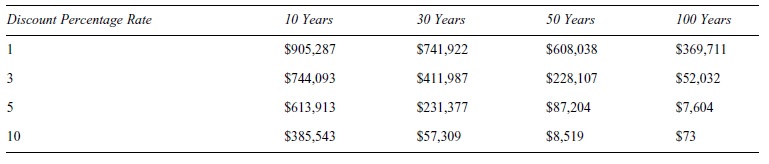
The actual discount rate used in economic evaluation often has a major impact on the result. Consider Table 1, which shows the present value of $1 million in 10, 30, 50, and 100 years in the future with discount rates of 1%, 3%, 5%, and 10%. As an example, with a discount rate of 1%, the present value of $1,000,000 occurring in 10 years is $905,287. The present value if using a discount rate of 5% is instead $613,913.

Table 1 can be used to show how important the discount rate is for the discussion regarding what to do about global warming. The predicted costs of global warming are assumed to lie quite distantly in the future. The effect of different discount rates will be relatively larger the more distant in the future the benefit or cost will take place. An environmental cost of $1 million occurring in 100 years is equal to only $7,604 in present value if using a discount rate of 5%. If using a discount rate of 1%, it is $369,711. A policy that would be paid for today to eliminate this cost in 100 years would be increasing social welfare if it cost less than $7,604 using the higher discount rate (5%) or would be increasing social welfare if it cost less than $369,711 using the lower discount rate (1%). Hence, it is obvious that the conclusion on how much of current GDP we should spend to decrease costs of global warming occurring in the distant future will be highly dependent on the chosen discount rate used in the cost-benefit analysis.

In 2006, a comprehensive study on the economics of climate change was presented by the British government: the Stern Review (Stern, 2007). The review argues that the appropriate discount rate for climate policy is 1.4%. Stern argues that because global warming is an issue affecting many generations, the pure time preference (p) should be very low (0.1), and he assumes an income elasticity (m) of 1 and a growth rate (g) of 1.3; this implies SDR = 0.1 + 1 x 1.3 = 1.4. This is a relatively low discount rate compared to what most governments recommend for standard cost-benefit analyses around the world for projects with shorter life spans than policies to combat global warming. The Stern Review has also been criticized by other economists, who argue that such a low discount rate is not ethically defensible and has no connection to market data or behavior (Nordhaus, 2007). Weitzman (2007) argues that a more appropriate assumption is that p=2, m = 2, and g = 2, which would give a social discount rate of 6%. The debate about the correct social discount rate has been a very public question in discussions about global warming policy—that is, how much, how fast, and how costly should measures taken today to reduce carbon emissions be?

Table 1.   Present Value of $1 Million Under Different Time Horizons and Discount Rates

There really exists no consensus regarding the correct discount rate, and there probably never will. Different government authorities around the world propose different social discount rates. The European Union demands that cost-benefit analyses be conducted for projects that imply important budget consumption, and the European Commission proposes a social discount rate of 5%. In the so-called Green Book in the United Kingdom, a social discount rate of 3.5% is proposed. In France, the Commisariat Général du Plan proposes a discount rate of 4%. In the United States, there are somewhat different proposals for different sectors, but the Office of Management and Budget recommends a social discount rate of 7% (Rambaud & Torrecillas, 2006). Several of the recommendations are also indicating that the social discount rate should be dependent on the time horizon of the project; in the United Kingdom, the social discount rate is proposed to be 3.5% for year 0 to 30, 3% for year 31 to 75, and decreasing down to 1% for policies with a life span of more than 301 years.

Sensitivity Analysis

There are often large uncertainties in a cost-benefit analysis, regarding parameter estimates of benefits and costs. It has been shown that, especially for large projects, costs are often underestimated and benefits are sometimes exaggerated, making projects look more beneficial than they actually are (Flyvbjerg, Holm, & Buhl, 2002, 2005). These types of uncertainties need to be explicitly discussed and evaluated in the analysis. One common approach to deal with uncertainty in a cost-benefit analysis is to perform sensitivity analyses. There are different approaches regarding how to conduct a sensitivity analysis. Partial sensitivity analysis involves changing different parameter estimates and examines how it affects the net present value of the policy. Examples include using different discount rates and different parameter values of the value of a statistical life. Another approach is the so-called worst- and best-case analysis. Imagine that the benefits are uncertain but that an interval can be roughly estimated—for example, the benefit of improving environmental quality will be in the interval $100,000 to $150,000. A worst-case analysis implies taking the lowest bound of all beneficial parameter estimates. A best-case analysis implies the opposite. These types of sensitivity analyses may be interesting for a risk-averse decision maker and also give information about the lowest benefit (or largest loss) for a given project.

The downside to partial sensitivity analysis and worst-and best-case scenarios is that they do not take all available information about the parameters into consideration. Further, they do not give any information about the variance of the net present value of a project. For example, if two projects give similar net present value, decision makers may be more interested in the project with the lowest variance around the outcome. This requires the use of Monte Carlo sensitivity analysis. This is based on simulations where economists make assumptions about the statistical distribution of different parameters and perform repeated draws of different parameter values, each leading to a different net present value. This can give an overview of the distribution of the uncertainty of the project. A standard approach to visually describe the results from a Monte Carlo sensitivity analysis is to display the results in a histogram that shows mean net present value, sample variance, and standard error.

An Application

To end this overview, a cost-benefit analysis of the Stockholm congestion charging policy is described (Eliasson, 2009). The Stockholm road congestion charging system is based on a cordon around central parts of Stockholm (capital of Sweden), with a road toll between 6:30 a.m. and 6:30 p.m. weekdays (higher charge during peak hours). The aim with the charging system is to reduce congestion and increase the reliability of travel times. Positive effects on safety and the environment are also expected. The cost-benefit analysis has the particular advantage of being based on observed traffic behavior, rather than simulations and forecasts (this is possible because the charging system was introduced during a trial period of 6 months). Using the six steps in a cost-benefit analysis as outlined in the introduction:

1. The first step involves defining the relevant population. The Stockholm congestion charging policy is mainly relevant for the population in the region of Stockholm, but because the cost-benefit analysis is based on actual behavior and data, it will therefore include benefits and costs of users of the roads in Stockholm, which will include various types of visitors as well. Hence, the relevant population is all the users of the roads.
2. The second step in a cost-benefit analysis is to identify the relevant consequences associated with the policy. The following main benefits are associated with the policy:

(a) reduction in travel times due to decreased congestion, (b) increased reliability in travel times, (c) reductions of carbon dioxide and health-related emissions due to the decrease in traffic volume, and (d) increased road safety due to decrease in traffic volume. It could be hypothesized that the system would have effects on decisions where to locate, the regional economy, and retail sales, but it has been judged that these effects will be very small. Negative effects are (a) investment and startup costs, and (b) yearly operation costs.

3. The third step in the cost-benefit analysis is to monetize all the benefits and costs associated with the policy. Table 2 summarizes the consequences and shows their monetary benefits and costs. Some of the smaller benefits and costs in the analysis are not described here; refer to the reference for a more detailed description.

Table 2.   Annual Benefits and Costs of the Stockholm Road Charging System

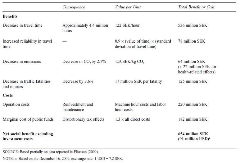
Table 2 shows the annual benefits and costs of the system. The magnitude of the effects on travel time, standard deviation of travel time, and so on is based on large computer estimations of the traffic measurements on 189 links to calibrate origin-destination (OD) matrices for the case with and without the charging system. The investment cost is not listed in Table 2 but was estimated at 1.9 million SEK.

4. The next step consists of calculating the net present value of all benefits and costs based on the annual estimates. It is not obvious which time horizon should be used for the project, but technical data and past experience indicated that it was reasonable to make a conservative assumption that the system would have an economic life span of 20 years. Hence, the benefits and operating costs in year 2, 3, … , 20 have to be discounted to a present value. The Swedish National Road Administration argues that the social discount rate should be 4%. Hence, the present value of the net social benefits in year 20 is 654 / (1.04)20 = 298 million SEK. These calculations are performed for benefits and costs in years 1 through 20.
5. Discount all annual benefits and costs to present values, as in Step 4, showing that the total social surplus (after deducting the investment costs) is approximately

6.3 billion SEK (approx. $800 million). Expressing it as a payback estimate, this means that the policy will take 4 years before the investment costs are fully repaid. It is also explicitly discussed that some consequences were deemed too difficult to include in the calculations, such as the effects on noise, labor market, time costs for users, quicker bus journeys, and so on.

6. The sixth step in a cost-benefit analysis is to perform a sensitivity analysis. In this aspect, there is little done in the described analysis. One reason for this is that the actual estimates of the consequences as performed using OD matrices are very time consuming, which more or less implies that because of practical limitations, only one main estimation can be performed. A simple sensitivity analysis is performed assuming increasing benefits over the time horizon. But if any improvement to the cost-benefit analysis should be suggested, it would be to conduct a more detailed sensitivity analysis. The quite straightforward conclusion of the cost-benefit analysis, even though it should have included sensitivity analyses to satisfy our full requirements, is that social welfare will increase because of the charging system.

Conclusion

How should we evaluate a proposed public policy or regulation? A cost-benefit analysis is an approach that includes all relevant consequences of a policy and compares, in monetary units, benefits with costs. If benefits outweigh the costs, the policy is said to increase social welfare. Social welfare is defined using the Hicks-Kaldor criterion, which states that a policy increases welfare if the winners from the policy can compensate the losers from the policy and still be better off than if the policy is not implemented.

To conduct a cost-benefit analysis, one must identify consequences and express them in a monetary metric so that all consequences can be compared in the same unit of measurement. If benefits and costs arise in the future, they should be discounted to present value using a social discount rate. Finally, given the uncertainties involved with estimating consequences of a policy or regulation as well as uncertainties with the monetary estimates of the consequences, a proper cost-benefit analysis should include sensitivity analyses to show how robust the result is.

Finally, considering the definition of social welfare as usually applied in cost-benefit analysis (Hicks-Kaldor criterion), the typical cost-benefit analysis of a project or regulation estimates the effect on economic efficiency. Therefore, even though a very important guide to decision making, in most applications, cost-benefit analysis is often seen as one of several guides to the decision making process. Especially in political decision making, there will be other effects of interest, such as effects on income distribution and geographical distribution of benefits.

Bibliography:

1. Bateman, I. J., Carson, R. T., Day, B., Hanemann, N., Hett, T., Hanley, N., et al. (2004). Economic valuation with stated preference techniques: A manual. Cheltenham, UK: Edward Elgar.
2. Broome, J. (1978). Trying to save a life. Journal of Public Economics, 9, 91-100.
3. Carson, R. T., & Groves, T. (2007). Incentive and informational properties of preference questions. Environmental and Resource Economics, 37, 181-210.
4. Cicchetti, C. J., Freeman, A. M., Haveman, R. H., & Knetsch, J. L. (1971). On the economics of mass demonstrations: A case study of the November 1969 march on Washington. American Economic Review, 61, 719-724.
5. Eliasson, J. (2009). A cost-benefit analysis of the Stockholm congestion charging system. Transportation Research Part A, 43, 46-480.
6. Fischhoff, B., & Frederick, S. (1998). Scope (in)sensitivity in elicited valuations. Risk, Decision, and Policy, 3, 109-123.
7. Flyvbjerg, B., Holm, M. K., & Buhl, S. L. (2002). Underestimating costs in public works projects: Error or lie? Journal of the American Planning Association, 68, 279-295.
8. Flyvbjerg, B., Holm, M. K., & Buhl, S. L. (2005). How (in)accurate are demand forecasts in public works projects? The case of transportation. Journal of the American Planning Association, 71, 131-146.
9. Harrison, G. W., & Rutström, E. E. (2008). Experimental evidence on the existence of hypothetical bias in value elicitation methods. In C. Plott & V Smith (Eds.), Handbook of experimental economics results (pp. 752-767). New York: Elsevier Science.
10. (2006). Deliverable 5 proposal for harmonised guidelines. Developing harmonised European approaches for transport costing and project assessment (Contract No. FP6-2002-SSP-1/502481). Stuttgart, Germany: 1ER.
11. Hurley, F., Cowie, H., Hunt, A., Holland, M., Miller, B., Pye, S., et al. (2005). Methodology for the cost-benefit analysis for CAFE: Volume 2: Health impact assessment. Available at http://www.cafe-cba.org/assets/volume_2_methodology_ overview_02-05.pdf
12. Kahneman, D., Knetsch, J. L., & Thaler, R. (1990). Experimental tests of the endowment effect and the Coase Theorem. Journal of Political Economy, 98, 1325-1348.
13. Krupnick, A., Alberini, A., Cropper, M., Simon, N., O’Brien, B., Goeree, R., et al. (2002). Age, health and the willingness to pay for mortality risk reductions: A contingent valuation survey of Ontario residents. Journal of Risk and Uncertainty, 24,161-186.
14. Nordhaus, W. (2007). A review of the Stern Review on the economics of climate change. Journal of Economic Literature, 45, 686-702.
15. Persson, S., & Lindqvist, E. (2003). Värdering av tid, olyckor och miljö vid vägtrafikinvesteringar—Kartläggning och modellbe-skrivning [Valuation of time, accidents and environment for road investments: Overview and model descriptions] (Rapport 5270). Stockholm, Sweden: Naturvârdsverket (Swedish Environmental Protection Agency).
16. Rambaud, S. C., & Torrecillas, M. J. (2006). Social discount rate: A revision. Anales de Estudios Econômicos y Empresariales, 16, 75-98.
17. Ramsey, F. (1928). A mathematical theory of saving. Economic Journal, 38, 543-559.
18. Rosen, S. (1974). Hedonic prices and implicit markets: Product differentiation in pure competition. Journal of Political Economy, 82, 34-55.
19. Soguel, N. (1994). Evaluation monetaire des atteinties a l’environment: Une etude hedoniste et contingente sur l’impact des transports [Economic valuation of environmental damage: A hedonic study on impacts from transport]. Neuchatel, Switzerland: Imprimerie de L’evolve SA.
20. Stern, N. (2007). The economics of climate change. Cambridge, UK: Cambridge University Press.
21. Weisbrod, B. A. (1964). Collective-consumption services of individual-consumption goods. Quarterly Journal of Economics, 78, 471-477.
22. Weitzman, M. (2007). A review of the Stern Review on the economics of climate change. Journal of Economic Literature, 45, 703-724.
23. Willig, R. D. (1976). Consumer surplus without apology. American Economic Review, 66, 589-597.
24. Viscusi, W. K. (1998). Rational risk policy. Oxford, UK: Oxford University Press.
25. Viscusi, W. K., & Aldy, J. E. (2003). The value of a statistical life: A critical review of market estimates throughout the world. Journal of Risk and Uncertainty, 27, 5-76.