Regression Discontinuity Design Research Paper

To many, the RD design seems counterintuitive. Using a cutoff to assign participants to the treatment and comparison groups creates a pretreatment group nonequivalence that seems like it should lead to selection bias. But while the design does induce initial nonequivalence, it does not necessarily lead to biased treatment effect estimates. Instead of assuming pretreatment equivalence in measured and unmeasured means and variances—as with the randomized experiment—in the absence of a treatment effect the RD design requires the two groups to be equivalent in their pre–post regression functions. This assumption can be tested.

The major attraction of RD designs is that they can be used to estimate the effects of treatments given to those who most need or deserve them, provided that need or merit is determined as a qualification score on the assignment variable (i.e., the cutoff) and nothing else. Because the design does not require some needy individuals being assigned to a no-treatment group, it has ethical advantages over experiments for assessing treatment effects.

2. History

The RD design was first used in psychology by Thistlethwaite and Campbell (1960) and was first discussed in detail in Campbell and Stanley (1963). It has been repeatedly reinvented—by the economist Goldberger (1972), the statistician Rubin (1977), the educators Tallmadge and Horst (1976), and by the public health researchers Finkelstein et al. (1996). Despite such independent reinvention, the RD design has not been used much outside of compensatory education where students scoring below some predetermined cutoff value on an achievement test are then assigned to remedial training (Trochim 1984). But it has also been used to study how unemployment benefits influence recently released prisoners (Berk and Rauma 1983) and how different levels of incarceration affect those in prison (Berk and de Leeuw 1999). A variation was also used to study how class size affects test scores (Angrist and Lavy 1999).

The low frequency of published examples may be due to several factors. One is its recency. Another is that RD designs require administrators to assign participants to conditions solely on the basis of quantitative indicators, restricting the role of judgment, discretion, or favoritism. Finally, understanding the design depends on some familiarity with regression analysis, making the strategy difficult to convey to nonstatistical audiences.

3. The Basic RD Design Structure

Simulated data for an RD design are shown in Fig. 1. It depicts the example of a compensatory treatment— perhaps a reading program designed to help students who initially score poorly (defined as below the cutoff) on a standardized reading measure. The figure depicts the standard bivariate plot of post-test and pretest for 500 simulated participants. Data points for the treatment recipients are represented with ‘+ ’ while the comparison cases are ‘o.’ The cutoff value in this example occurs at the middle of the pretest distribution (pretest = 50) and is indicated by the vertical line. All students scoring below 50 are defined as needing compensatory training and get the treatment, while the remainder (i.e., those to the right of the cutoff) are assigned to the comparison group.

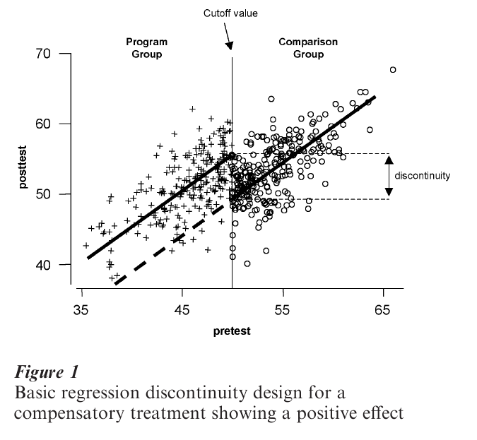
The solid lines represent the straight-line regression of post-test on pretest for each group. In the absence of a treatment effect, the critical assumption is that the regression line in the comparison group would continue to the left of the cutoff into the treatment group region, as indicated by the heavy dashed line. That is, if the reading program does not work, then the observed treatment group regression line would be where the dashed line is. The fact that the observed treatment group line is displaced from this ‘expected’ line suggests a treatment effect—treatment group participants scored higher on the post-test (i.e., vertically) than would have been predicted from the comparison group pre–post relationship. The size of the treatment main effect is estimated as the vertical jump or discontinuity between the regression lines at the cutoff. Assuming that higher scores on both measures indicate better performance, one can conclude from the figure that the treatment improved participant performance by the amount of the vertical discontinuity.

In experimental designs one assures through random assignment or otherwise that the treatment and comparison groups are initially equivalent. Otherwise, post-treatment differences can be attributed to the intervention. In the RD design one obviously does not expect this kind of equivalence. Instead, it is assumed that the relationship between the assignment variable and the outcome is equivalent for the two groups—that is, the same continuous regression line describes both groups. Thus, interpretation of the RD design depends mostly on two factors: (a) that no alternative cause operates at or near the cutoff; and (b) that we can perfectly model the pre–post relationship. These issues constitute the major problems in the statistical analysis of the RD design, particularly the second one.

4. Design Considerations And Variations

4.1 Selection Of The Cutoff

The choice of cutoff value can be made solely on the basis of available resources. If a program can only handle 25 persons and 70 apply, then a cutoff point can be selected that distinguishes the 25 most ‘needy’ persons from the rest. The cutoff can also be chosen on substantive grounds. If the assignment measure is an indication of severity of illness measured on a 1–7 scale, relevant experts might contend that all those scoring 5 or more are ill enough to deserve treatment. So, a theoretically justified cutoff of 5 is used.

4.2 Assignment Variations

While the use of a pretreatment cutoff value distinguishes the RD design, it is often difficult to implement. In many situations it does not appear to allow room for professional judgment or discretion. In fact, the design does not preclude incorporating such judgment so long as it can be quantified or explicitly accounted for when specifying the cutoff value.

Violation of the assignment rule leads to ‘misassignment.’ It seems to be most prevalent at scores around the cutoff and is often labeled as the ‘fuzzy’ RD design. Standard analyses will yield biased estimates of treatment effect in the fuzzy RD case. While statistical procedures for dealing with mis-assignment have been suggested (Trochim 1984), mis-assignment is better avoided if possible.

4.2.1 Multiple Cutoff Points. RD designs are not limited to a single cutoff value. In the absence of treatment the assumption is that the pre–post relationship can be described as a single continuous regression line extending over the entire range of the assignment scores. Even when multiple cutoff points are used, the comparison group’s pre–post relationship is still used as the counterfactual for projecting where other groups’ regression lines should be if there is no treatment effect.

The simplest multiple cutoff case involves two cutoff scorees. In this variant, persons scoring above the higher cutoff might be assigned to one treatment, those scoring below the lower cutoff to another, and those scoring within the cutoff interval might be controls. The assignment of treatments to each part of the assignment distribution can be made in many ways, including by random assignment.

Considerable work has been done on another way of ‘coupling’ the RD design to the randomized experiment. This is when individuals scoring in a range just above or below an originally selected cutoff value are randomly assigned to conditions, while those scoring further below and further above the cutoff are analyzed as from an RD design (Boruch 1973). Trochim and Cappelleri (1992) discuss four other ways of coupling random assignment to RD design features.

Multiple cutoff points are also involved in designs where the treatment is implemented a series of times (i.e., in phases), perhaps beginning with the most needy before successively giving it to those less needy. In the first phase, one uses a single cutoff value, assigning those most in need to the treatment and then measuring post-treatment performance. Then the cutoff value would be moved to include the next most needy group on the assignment measure. Eventually, everybody could receive the treatment, but in groups ordered by need and phase. This is particularly useful in organizations seeking to ‘roll-out’ a treatment over time, but eventually serving all.

4.2.2 Multiple Assignment Measures. The requirement of strict adherence to the cutoff criterion entails a single quantitative indicator. When this does not capture the degree of pretreatment need well, Trochim (1990) discusses two multivariate strategies. The first involves the use of several separate measures, each having its own cutoff value. This is most feasible when a prospective participant must meet the different cutoff criteria on measure 1 ‘and’ measure 2 ‘and’ measure 3, etc. Less feasible is an ‘or’ rule when assignment depends on meeting a fixed number of criteria from a larger set—say, 5 out of 10. The second involves assignment according to a new variable that is a composite of several individual measures. Using multiple measures this way can help incorporate more judgment into a quantitative assignment strategy.

4.3 Treatment Variations

When treatment comparisons are absolute, the control group receives no formal treatment or a placebo treatment. When they are relative, the comparison group receives an alternative treatment, very often the current treatment to which a novelty is to be compared.

An advantage of the RD design is that it enables assignment of progressively riskier treatments to those in greater need. Assume three treatment programs: the standard, plus two increasingly riskier experimental ones. It is then possible to have two cutoff points and to assign the riskiest treatment to the neediest patients, the least risky (i.e., standard) treatment assigned to the least needy, and the moderately risky treatment assigned to those falling between the two cutoffs. (If no a priori basis exists for making risk judgments, an alternative would be to use a single cutoff and to assign those least in need to standard treatment while randomly assigning those on the other side of the cutoff into one of the two experimental protocols.) RD designs are flexible for examining treatment variations.

5. Post-Treatment Measurement Variations

In RD designs, pre- and postmeasures do not have to be on the same or equivalent measures. For instance, one might assign persons to a health education treatment on the basis of household income but then examine its effects on attitudes towards health. The assignment variable is an economic indicator and the outcome is a cognitive one.

The RD design is not restricted to a single outcome, and for each post-treatment measure there can be a separate RD design and analysis. But it will often be useful to create an aggregate outcome or outcomes. For instance, we may have many knowledge items that are scaled to give a total and subtest scores for mathematical reasoning, computational skills, verbal reasoning, analogies, and so on. We might then conduct separate analyses for both the total score and each subtest.

Outcome measures need not be continuous normal variables. While such distributions facilitate RD analysis, they are not necessary for it. Thus, Berk and Rauma (1983) evaluated the effects of a California law that extended unemployment benefits to released prisoners who had not previously been eligible. In order to qualify, prisoners had to earn at least $1,500 working in the prison over the 12 months prior to release. Would extending these benefits reduce subsequent recidivism—a dichotomous outcome where 1 indicated recidivism and 0 staying out of prison? To analyze this outcome, Berk and Rauma (1983) relied on a linear random utility model related to the binary logit model. When continuous normal outcomes are not feasible, the analyst must specify a statistical model to account for the specified distributional form of the outcome.

5.1 Internal Validity

Internal validity refers to the degree to which causal inference is reasonable because all alternative explanations for an apparent treatment effect can be ruled out. The RD design is very strong with respect to internal validity because the process of selection into treatments is fully known and only factors that would serendipitously induce a discontinuity in the pre–post relationship at the cutoff can be considered threats. However, validity also depends on how well the analyst can model the true pre–post relationship so that underlying nonlinear relationships do not masquerade as discontinuities at the cutoff point.

5.2 Measurement Error

Stanley (1991) has argued that the RD design yields biased estimates of the treatment effect when the assignment variable is measured with error. Cappelleri et al. (1991) refuted this for situations with no interaction effects and Trochim et al. (1991) for the interaction case. The reason such error does not induce bias here although it does in quasiexperiments is that assignment to treatment is by the fallible assignment variable and not by some latent underlying selection process, as happens in quasiexperiments.

5.3 Statistical Power

It takes approximately 2.75 times as many participants in an RD design to achieve statistical power comparable to a simple randomized experiment (Goldberger 1972). When RD is combined with random assignment within an interval around this cutoff, 2.48 times the number of respondents are needed if 20 percent of participants are randomized; 1.96 times with 40 percent randomization; 1.46 with 60 percent; and 1.14 with 80 percent (Cappelleri and Trochim 1994, 1995).

6. Analysis

6.1 Assumptions Of RD Analysis

Five central assumptions must be made in order for responsible analysis of data from an RD design:

(a) The cutoff criterion. The cutoff criterion must be followed without exception. Otherwise, a selection threat arises and estimates of the treatment effect are likely to be biased.

(b) The pre–post distribution. The true pre–post distribution must be known and correctly specified as linear, polynomial, logarithmic, or the like. Reichardt et al. (1995) point out the difficulties in specifying the appropriate model, especially when some curvilinearity exists in the pre–post relationship.

(c) Comparison group pretest variance. There must be a sufficient range of pretest values in the comparison group to enable adequate estimation of the pre–post regression line for that group. Variability in the treatment group is also desirable, though not strictly required because one can project the comparison group line even to a single treatment group point.

(d) Continuous pretest distribution. Both groups must come from a single continuous pretest distribution. In some cases one might find intact groups that serendipitously divide on a measure so as to imply some cutoff (e.g., pents from two different geographic locations). But such naturally discontinuous groups must be used with caution.

(e) Treatment implementation. It is assumed that the treatment is uniformly delivered to all recipients— that is, they all receive the same dosage, length of stay, amount of training, or whatever. If not, it is necessary to model explicitly the treatment as implemented, thus complicating the analysis considerably.

6.2 A Model For The Basic RD Design

The model presented here is for the basic RD design. Given a pretest assignment measure, xi, and a post- treatment measure, y_i, the model can be stated as follows:

Where x_i = pretreatment measure for individual i minus the value of the cutoff, x₀ (i.e., x_i = x_i – x₀); y_i = post-treatment measure for individual i; z_i = assignment variable (1 if treatment participant; 0 if comparison participant); s = the degree of the polynomial for the associated x_i; β = parameter for comparison group intercept at cutoff x₀; β₁= linear slope parameter; β₂ = treatment effect estimate; β_n = parameter for the sth polynomial or interaction terms if paired with z; e₁ = random error.

The major hypothesis of interest is: H₀: β₂ = 0 tested against the alternative: H₁: β₂ = 0. This model estimates both main and interaction effects at the cutoff point in order to examine changes in means and slopes. It postulates a pre–post relationship that is polynomial at the cutoff. It also requires subtracting the cutoff score from each pretest score. The term x_i has a superscript tilde to indicate this transformation of the pretest xi. Finally, the model allows for any order of polynomial function (although certain restrictions are made in specifying the function as described below). Thus, the true pre–post relationship can in theory be linear, quadratic, cubic, quartic, and so on, or any combinations of these.

6.3 Model Specification

The key analytic problem is correctly specifying the model for the data—in this example, as a polynomial model. No simple or mechanical way exists to determine definitively the appropriate model. As with any statistical modeling, the RD analysis requires judgment and discretion and conducting multiple analyses based on different assumptions about the true pre–post relationship.

6.4 Steps In The Analysis

Recall what data the basic RD design provides on each unit. There is a pretest assignment value xi in the model. Knowing this and the cutoff value allows creation of a new variable, z_i, which is equal to 1 in the treatment group and 0 if not. Finally, there is a post- test score labeled y_i in the model. Given the variables x_i, z_i, and y_i, the steps to be followed in the polynomial analysis are:

(a) Transform the pretest. The analysis begins by subtracting the cutoff value from each pretest score, thus creating the term as in the model. This sets the intercept equal to the cutoff so that estimates of effect are made at the cutoff rather than at x_i = 0.

(b) Examine the relationship visually. It is important to determine whether there is any visually discernible discontinuity at the cutoff. It could be a change in level, in slope, or both. If a discontinuity is visually clear at the cutoff one should not be satisfied with analytic results that indicate no effect. However, if no discontinuity is apparent, variability in the data may be masking an effect and one must attend carefully to the analytic results.

The second thing to look for is the degree of polynomial that may be required as indicated by the overall slope of the distribution, but particularly in the comparison group part. A good approach is to count the number of flexion points (how often the distribution ‘flexes’ or ‘bends’). A linear distribution implies no flexion points, while a single flexion point could indicate a quadratic function. This information is used to specify the initial model.

(c) Create higher-order terms and interactions. De-pending on the number of flexion points, create transformations of the transformed assignment variable, x_i. The rule of thumb is that one goes two orders of polynomial higher than indicated by the number of flexion points. Thus, if the bivariate relationship appeared linear (i.e., no flexion points), one would want to create transformations up to a second-order (0 + 2) polynomial. The first-order polynomial already exists in the model (x_i) and so one would only have to create the second-order polynomial by squaring x_i to obtain x_i². For each transformation of x_i one also creates the interaction term by multiplying the polynomial by z_i. In this example there would be two interaction terms: x_iz_i and x_i²z_i. If there seem to be two flexion points in the bivariate distribution, one would then create transformations up to the fourth (2 + 2) power and their interactions. This rule of thumb errs towards overestimating the true polynomial function needed, for reasons outlined in Trochim (1984).

(d) Estimate the initial model. The true analysis can now begin. One simply regresses the post-test scores, y_i, on x_i, z_i and all higher-order transformations and interactions created in step (c) above. The regression coefficient associated with the z_i term (i.e., the group membership variable) is the estimate of the main effect of the treatment. If there is a vertical discontinuity at the cutoff it will be estimated by this coefficient. One can test the significance of the coefficient (or any other) by constructing a standard t-test. If the analyst correctly overestimated the polynomial function required to model the distribution at step (c), then the treatment effect estimate will be unbiased. However, by initially including terms that may not be needed in the true model, the estimate is likely to be inefficient— that is, standard error terms will be inflated and statistical significance underestimated. But if the coefficient for the effect is highly significant, it would be reasonable to conclude there is an effect. Interaction effects can also be examined. A linear interaction is implied by a significant coefficient for the x_iz_i term.

(e) Refining the model. The procedure described thus far is conservative, designed to reduce the chances of a biased treatment effect estimate even at the risk of increasing the error of the estimate (Trochim 1984). So, on the basis of the results of step (d) one might wish to attempt to remove apparently unnecessary terms and re-estimate the treatment effect with greater efficiency. This is tricky and should be approached with caution lest it introduces bias. One should certainly examine the regression results from step (d), noting the degree to which the overall model fit the data, the presence of any insignificant coefficients, and the pattern of residuals. One might examine the highest-order term in the current model and its interaction. If both coefficients are nonsignificant, and the goodness-of-fit measures and pattern of residuals indicate a good fit, one might then drop these two terms and re-estimate the model. One would repeat this procedure until either: (i) all of the coefficients are significant; (ii) the goodness-of-fit measure drops appreciably; or (iii) the pattern of residuals indicates a poor fit.

6.5 Analyses With Multiple Cutoff Points

The basic model described above can be applied directly when multiple cutoff points are used and random assignment is used within cutoff intervals. If assignment within intervals is nonrandom, one must also address the potential for selection bias in the analysis. When multiple cutoffs are used to distinguish separate treatments (i.e., multiple treatments are not assigned within the same cutoff interval), one would have to construct multiple treatment assignment variables for the analytic model (e.g., z₁, z₂, z₃) and all necessary interaction terms. Clearly, as more cutoffs and groups are added, model specification becomes more complex.

6.6 Analyses With Multiple Assignment Measures

Imagine having multiple measures, each with its own cutoff. Each assignment measure is then transformed by having its own cutoff value subtracted from it to create xi. The analysis would then include all trans- formed assignment measures, group membership, higher-order terms, and interactions. For the simple first-order (or linear) case, one could use the model:

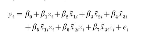
This model does not include any two-way assignment variable interactions terms (e.g., β_ix_1ix_2i or β_ix_1ix_2iz_i) or any three-way terms (e.g., β_ix_1ix_2ix_3i and β_ix_1ix_2ix_3iz_i) but such an assumption may be reasonable where primary interest is in estimating β₁, the treatment effect, and not interactions. Clearly, though, the use of multiple assignment variables with higher order polynomial models will quickly lead to an unwieldy analysis.

The situation is simpler when multiple assignment variables are rescaled to reflect ‘number of assignment variables on which a person meets the criterion’ (e.g., on 5 of 10). This number then becomes the xi variable and one would conduct the basic analysis described earlier. When multiple assignment variables are combined into a single index, the analysis is also a straightforward application of the basic procedures described initially.

7. Conclusions

From a methodological point of view, inferences drawn from a well-implemented RD design are considered comparable in internal validity to conclusions from randomized experiments. However, the lower statistical efficiency of RD designs, and the resulting sample size demands, may limit the design’s utility. From an ethical perspective, RD designs are compatible with the goal of getting the treatment to those most in need. It is not necessary to deny the treatment from potentially deserving recipients simply for the sake of a scientific test. From an administrative viewpoint, the RD design may be directly usable when allocation formulas are the basis for assigning treatments or programs.

With all of these considerations in mind, the RD design must be used judiciously. In general, the randomized experiment is still the first method of choice when assessing causal hypotheses (Cappelleri and Trochim 2000). However, where they are ruled out as impractical, the RD design should be considered as a practical alternative.

Bibliography:

1. Angrist J D, Levy V 1999 Using Maimonides’ Rule to estimate the effect of class size on scholastic achievement. Quarterly Journal of Economics 114: 533–75
2. Berk R A, de Leeuw J 1999 An evaluation of California’s Inmate Classification System using a generalized regression discontinuity design. Journal of the American Statistical Association 94: 1045–52
3. Berk R A, Rauma D 1983 Capitalizing on nonrandom assignment to treatments A regression discontinuity evaluation of a crime control program. Journal of the American Statistical Association 78: 21–8
4. Boruch R F 1973 Regression-discontinuity designs revisited. Unpublished manuscript. Northwestern University
5. Campbell D T, Stanley J C 1963 Experimental and quasiexperimental designs for research on teaching. In: Gage N L (ed.) Handbook of Research on Teaching. Rand McNally, Chicago (Also published as Experimental and Quasi-experimental Designs for Research. Rand McNally, Chicago, 1966)
6. Cappelleri J C, Trochim W M K 1994 An illustrative statistical analysis of cutoff-based randomized clinical trials. Journal of Clinical Epidemiology 47(3): 261–70
7. Cappelleri J C, Trochim W M K 1995 Ethical and scientific features of cutoff-based designs of clinical trials: A simulation study. Medical Decision Making 15(4): 387–94
8. Capelleri J C, Trochin W 2000 Cutoff In: Chow S-C (ed.) Encyclopedia of Biopharmaceutical Statistics. Marcel Dekker, New York, pp. 149–56
9. Cappelleri J C, Trochim W M K, Stanley T-D, Reichardt C S 1991 Random measurement error does not bias the treatment effect estimate in the regression-discontinuity design: I. The case of no interaction. Evaluation Review 15(4): 395–419
10. Finkelstein M O, Levin B, Robbins H 1996 Clinical and prophylactic trials with assured new treatment for those at greater risk. 2. Examples. American Journal of Public Health 86: 696–705
11. Goldberger A S 1972 Selection bias in evaluating treatment effects: Some formal illustrations. Discussion Papers, 123–72. University of Wisconsin, Madison, WI
12. Reichardt C S, Trochim W M K, Cappelleri J C 1995 Reports of the death of regression-discontinuity analysis are greatly exaggerated. Evaluation Review 19(1): 39–63
13. Rubin D B 1977 Assignment to treatment on the basis of a covariate. Journal of Educational Statistics 2: 1–26
14. Stanley T D 1991 ‘Regression-discontinuity design’ by any other name might be less problematic. Evaluation Review 15(5): 605–24
15. Tallmadge G K, Horst D P 1976 A Procedural Guide for Validating Achievement Gains in Educational Projects. Office of Education, Washington, DC
16. Thistlethwaite D L, Campbell D T 1960 Regression-discontinuity analysis: An alternative to the ex post facto experiment. Journal of Educational Psychology 51: 309–17
17. Trochim W M K 1984 Research Design for Treatment Evaluation: The Regression-Discontinuity Approach Program. Sage, Beverly Hills, CA
18. Trochim W 1990 Regression-discontinuity design in health evaluation. In: Sechrest L, Perrin E, Bunker J (eds.) Research Methodology: Strengthening Causal Interpretations of Nonexperimental Data. US Dept. of HHS, Agency for Health Care Policy and Research, Rockville, MD, pp. 119–39
19. Trochim W M K, Cappelleri J C 1992 Cutoff assignment strategies for enhancing randomized clinical trials. Controlled Clinical Trials 13: 190–212
20. Trochim W M K, Cappelleri J C, Reichardt C S 1991 Random measurement error does not bias the treatment effect estimate in the regression-discontinuity design: II. When an interaction effect is present. Evaluation Review 15(4): 571–604