Quantitative Cross-National Research Methods Research Paper

Quantitative nation comparisons will, however, inevitably face a number of tradeoffs; some more serious than others. One is that the capacity for broader generalization that quantification permits is bought at the price of less attention to the contextual reality of individual nations. The uniqueness of a nation’s culture, historical heritage, and endemic logic is lost easily when all we actually observe are a few indicators. Moreover, these indicators may mean somewhat different things in the unique context of specific countries (Ragin 1987). Scholars are frequently quite sensitive to this issue and so attempt to embed their statistical analyses within the histories and social uniqueness of the countries being studied. Also, as Ragin (1994) argues and empirically demonstrates, Boolean analysis can help overcome this dilemma by enabling us to build conjunctural models with very few cases and to analyze nonevents. But the approach is somewhat circumscribed. It needs to be guided by strong theory and background knowledge, its applicability is limited to relatively few cases, and it may be biased in favor of corroborating nonadditive, conjunctural models.

A second constraint has to do with the often limited number of observations available. This is especially true of studies of advanced (OECD) democracies where the N rarely exceeds 25. In broader worldwide comparisons, however, the N approaches 200. Many researchers attempt to supplement the paucity of nations by collecting longitudinal data on each nation, as with pooled cross-sectional and time series analyses. A 20-year time series for 20 countries yields 400 observations; a 20-year time series for 200 nations yields 4,000. As ever, longer data series for individual countries become available, the small N problem will gradually diminish.

Small samples do not necessarily pose problems of statistical inference, especially when the substantive theory is strong. They do, however, limit what statistical tools can be brought to bear. Fearon (1991) argues that the smaller the sample size, the greater is the need to make counterfactuals explicit—in other words, to tighten the theoretical formulation about the precise conditions that will (or will not) produce an outcome. Vague theory implies uncertainty about the number of contending explanations (which can grow very large) and about their mutual relationship within a causal order. The consequences of this include causal mispecification, multi-colinearity and large error terms. The last two of these can only be managed by having more observations. Without them, estimations are likely to yield results that are not robust. The less ambiguous the theory, the less the need for large N’s. Small N’s are, therefore, an especially acute problem in disciplines without a firm theoretical architecture, like sociology or political science. Western (1998a) argues that Bayesian estimation, by allowing for greater uncertainty, produces more robust results when N’s are few, theory vague, and explanations are many.

Small N’s can even hold advantages, because a limited nation sample implies that the researcher can gain more easily maximum advantage from diagnostic scrutiny of the residual plots. A set of systematic outliers, for example, can be easily identified in terms of their nationhood, and any good comparativist should be able to pin down what variable(s) drives their deviance from the fitted regression line. Diagnostics on small samples can approach the advantages of in-depth case studies.

The constraints imposed by small samples are generally well known to researchers. There are additional problems inherent in quantitative national comparisons that are both more generic and potentially more serious, but also less recognized. Chief among these are issues related to: qualitative and limited dependent variables, the potential for selection bias, possible lack of independence between observations and, finally, the question of endogeneity of variables.

2. Qualitative And Limited Dependent Variables

Many dependent variables in cross-national research are either qualitative (assuming discrete values) or limited (they assume continuous values within some range). The choice whether to measure a variable in a qualitative or continuous way is often controversial. Bollen and Jackman (1989), for example, argue that difficulties in classifying some political regimes speak in favor of using continuous scales because ‘Dichotomizing democracy blurs distinctions between borderline cases.’ In contrast, Przeworski et al. (in press) prefer to treat regimes dichotomously or multinomially.

When the dependent variable is either qualitative or limited, we need to use nonlinear models. Whether we give political regimes the values of 0–1 (as do Przeworski et al. in press) or 1–100 (as does Bollen 1980), it remains that the value on the dependent variable cannot exceed its maximum when the independent variable(s) tend to infinity, and it cannot fall below its minimum when these variables tend to infinity. Linear models, at best, can provide an approximation within some range of the independent variables.

The standard model when the dependent variable is multinomial is

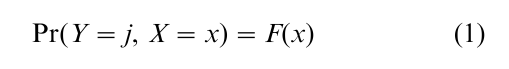
where j = 0, 1, … , J 1 and F is the cumulative distribution function. Since such models are covered by any standard textbook we need not present them here. Such models can be applied to panel data unless the number of repeated observations is large.

‘Event history analysis’ is one particular class of nonlinear models applied in cross-national research. In such models the dependent variable is an event, such as a revolution, regime transition, or a policy adoption. The general model is

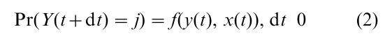
Most often, such models can be conveniently estimated as

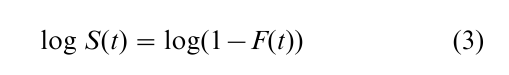
where S(t) is the survival function, or the probability that an event lasts beyond time t, and F(t) is the cdf. For dichotomous dependent variables, logit and probit give very similar results.

For multinomial variables, it is often assumed that the errors are independent across the values of the dependent variable, which leads to a logit specification. But this implies a strong assumption, namely the irrelevance of independent alternatives that rarely holds in practice. Multinomial probit, in turn, requires computing multiple integrals, which was until recently computationally expensive. Alternatives would be semiand nonparametric methods.

The distributions that are commonly used in estimating survival models include the exponential, Weibul, logistic, and Poisson distributions. But, except for the Weibul and exponential, it is very difficult to distinguish statistically between such distributions.

Methods for studying qualitative dependent variables are now standard textbook fare, but what warrants emphasis is that the traditional distinction between ‘qualitative’ and ‘quantitative’ research is becoming increasingly obsolute. Phenomena such as social revolutions may be rare, but this just means they occur with a low probability. They can, nevertheless, be studied systematically using maximum likelihood methods.

3. The Problem Of Selection Bias

In comparative research we are often interested in the effect of some systemic feature, institution, or policy on some outcome. Examples include the effect of labor market institutions on unemployment, the effect of political regimes on economic growth, or the effect of electoral rules on the number of political parties.

In such cases, the question is how some feature of X affects some outcomes Y in the presence of conditions Z, or PR (Y, X, Z), where the hypothesis is that y = f(x). The generic problem is how to isolate the effects of X and Z on Y.

If sampling is exogenous (i.e., the probability of observing any y is independent of z), the pr(Y = yz) = pr(y), and standard statistical methods can be used. But if pr(Y = yz) is different under different conditions Z, sampling is endogenous and the assumptions of the standard statistical model are violated.

To exemplify the problem: suppose we want to know the impact of political regimes on economic growth. We observe Chile in 1985 (Z ), which was a dictatorship (X ), in which case per capita income declined at the rate of Y = – 2.26. To assess the effect of political regimes, we need to know what would have been the rate of growth (Y ) in Chile had it been a democracy. This cannot be answered with the available observations because Chile in 1985 was indeed a dictatorship. The comparativist in such a case would proceed quasi-experimentally, and look for a case that matches Chile in all aspects except authoritarianism. In this way one would compare an authoritarian with a democratic ‘Chile.’

But what if Chile’s status as a dictatorship in 1985 was due to some factors that also affected its economic performance? This could be because growth itself influences the survival of regimes; a country’s level of development may be associated both with regime selection and growth; some unobservable factors (say ‘enlightened leadership’ or, perhaps, measurement error) may be common to both variables. Whatever the underlying selection mechanism, the basic consequence is that there will be cases without a match, and this implies that our inferences will be biased.

The problem raised by nonrandom selection is how to make inferences from what we observe to what we do not. It is a problem of identification (Manski 1995). For what do we know when we observe Chile as a dictatorship in 1985? We observe the fact that, given conditions Z, the Chilean regime (X ) is a dictatorship. We also know its rate of economic growth, given that it is a dictatorship under conditions Z. We do not observe, however, its rate of growth as a democracy under conditions Z. The issue is one of counterfactual observations: the rate of growth that an observation with Z = zi, observed under dictatorship, would have had under democracy. We do not know what this value is and, hence, we face under-identification.

What we need to know are two distributions, P(Y = y, x = j, Z ) and P(Y = y, x = k, Z ), and their expected values, where we now think of the possible values of X more generally as j, k = 0, 1, 2,… ,N. The first is the distribution of Y in the entire population if all cases were observed as dictatorships; the second is the distribution of Y in the entire population if all cases were observed as democracies. Clearly, if we want to know the impact on y of being in states x, we need to determine the difference between these two distributions, conditional on z.

It may seem strange to refer to the ‘population’ as including unobserved cases. But in order to compare the effects of states x on the performance of an individual case characterized by a zi, we must allow the case to be potentially observable under the full range of X. We observed this case as X = j, but must also imagine the possibility that it would have been Xj. We must think in terms of a ‘superpopulation’ consisting of a continuum of potential cases. The actual sample is then regarded as having been drawn by ‘nature’ from this superpopulation.

If the actual population is an exogenous sample of the potential one, any multivariate combination (xi, zi) can be drawn with a positive probability. Such exogenous sampling allows us to isolate the effect of x on y given z, that is, to ‘control’ for z the effects of x on y. If the sample is exogenous, we can ‘match’ pairs (xi = j, zi) and (xi = k, zi). But if sampling is endogenous, there will be some cases without a ‘match’: some of the xi’s will not have support. Where we have nonrandom selection, quasi-experimental comparisons fail regardless of the number of observations.

The methods to correct for selection bias consist of constructing counterfactuals, that is, of filling the unobserved supports of the distribution Y for all X. Following Heckman (1979), when sampling is not random, the regressions y = f (x, z) suffer from omitted variable bias. When such regressions are estimated on the basis of the observed sample, the variable that is omitted is the expected value of the error in the equation that specifies how the observations are selected into the sample

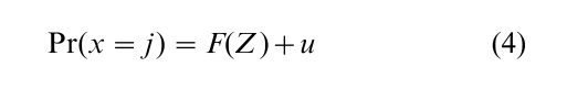
if

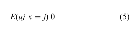
then

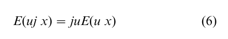
where ju is a regression coefficient of uj on u.

Finally, E(ux = j) = j, where the j’s are the inverse Mill ratios, or the hazard rates. Since we know that Yj is observed when x = j, we can write the expected values in the observed sample as

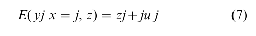
Note that if this equation is estimated on the basis of the observed sample, the variable j is omitted from the specification.

We can now see why controlling for the variables that enter both into selection and outcome equations may indeed worsen the selection bias. Following Heckman (1988), we distinguish first between selection on observables and on unobservables. Selection on observables occurs when the expected covariance E(uju z) = 0, but once the observed variables Z are controlled for it vanishes, so that E(uju z) = 0. Selection is on unobservables when E(uju) 0 and E(uju z) 0, which means that controlling for the factors observed by the investigator does not remove the covariance between the errors in the outcome and the selection equations. Now note that the regression coefficient ju = cov(uju)/var(uj). If selection is on unobservables, controlling for some variable x in the outcome equation may reduce the error variance uj without equally reducing the covariance uju. Hence, the coefficient on the omitted variable will be larger and the bias will be exacerbated.

In short, the expected values of the observed cases will be biased because they co-vary with the variable which determines which cases are observed. If selection is exclusively on observables, this bias can be corrected by traditional controlling techniques. But if it is on unobservables, such controls only worsen the bias.

Correcting for selection bias is not uncontroversial. It has been found that corrections for selection are not robust, but are highly sensitive to relatively minor changes in assumptions about distributions (Goldberger 1983). Others have found that some estimation methods fail to correct for this bias and may even exacerbate it (Stolzenberg and Relles 1990). As Heckman (1988) argues, the quandary we face is that different methods of correcting for selection bias are robust if there is no bias to begin with; if there is, there is no guarantee that the methods are robust.

The logic of the problem is similar whether we study large or small N’s. When de Toqueville concluded that revolutions do not bring about social change, the reason might be that they occur only in countries where it is difficult to change society. Even when N 1, the issue of selection bias does not disappear: The French revolution in 1789 may have been caused by the same conditions that made social change so difficult. It is possible that a revolution in a country where social relations are easier to change would have provoked change. But then a revolution would not have been necessary.

Comparativists who conduct case studies cannot benefit from statistical distributions to generate the counterfactuals. Yet, as in all cases of comparison the problem remains and it should, therefore, be standard practice to ask counterfactual questions of one’s case or cases.

4. The Problem Of Independence

Statistical inference must assume that the observations on a variable are independent one of the other. Is country A’s performance truly independent of what happens in country B? Is what happens at t + 1 independent of events in t? Usually not, and this implies the need for corrective procedures. In most cases, however, rigorous correction will entail that the de facto N (nations or years) diminishes; in some instances, statistical dependency cannot be resolved at all.

Cross-sectional analysis almost invariably assumes that nations and their properties (say budgets or institutions) are independent one of the other. This should not be assumed. We know that the Scandinavian countries have a shared history, deliberately learning from each other through centuries, thus creating similar institutions and path dependencies. The same goes for Austria and Germany, for Belgium and The Netherlands and, arguably, for all the Anglo-Saxon nations. World samples have a similar problem: Japan’s long hegemony in East Asia will have influenced Korean society; Confucianism has had a pervasive influence throughout the region. Similar stories are easily told for Latin America and Africa. If the World is a set of nation clusters, the real N is not 20-odd OECD countries or 150-odd World nations.

When nations form families, but are treated as if they were all unique and independent, we are likely to get biased coefficients and, very probably, unequal error variance (heteroskadicity). Sweden alone will drive the regression line in just about any welfare state analysis, and when also Denmark and Norway are treated as discrete observations, the bias is multiplied in so far as all three in reality form part of the same political family (‘Scandinavia’). Diffusion effects that operate between members of a nation–cluster can also result in heteroskadistic disturbance in the cross-section. Such can be corrected by, for example, adding a variable that captures the common underlying property that drives the disturbance (say, a dummy for being ‘Scandinavia’) but, again, this correction absorbs precious degrees of freedom in a small N study and, substantively, amounts to reducing the three nations to one observation.

Lack of independence in a time-series is normally taken for granted, since this year’s budget or election outcome is almost inevitably related to last year’s budget or the previous election. The standard assumption is a first-order (AR1) serial correlation. In comparative research virtually all time-series applications are pooled with cross-sections. But, where N’s are very small, one may as well simply compare across individual time-series estimations, as do Esping-Andersen and Sonnberger (1991). Time-series are meant to capture historical process. Yet as Isaac and Griffin (1989) argue, they easily end up being ahistorical.

Pooling cross-sectional with time-series data (panel regressions) has become very widespread, especially in studies of the limited group of advanced (OECD) societies. In many cases, the panel design is chiefly cross-sectional (more nations than years); others are temporally dominated (for a discussion, see Stimson 1985). Panel models are especially problematic because they can contain simultaneous diachronic and spatial interdependence and, worse, the two may interact. The standard method for correcting contemporaneous error correlation (GLS) applies only where the t’s well exceed nations (which is rare). The consequence is that t-statistics are overestimated, errors underestimated, and the results may therefore not be robust (Beck and Katz 1995). The Beck and Katz (1995) procedure can correct for temporal and cross-sectional dependency one at a time, but if the two interact, no solution exists. See also Beck et al. (1998) for an application to maximum likelihood estimation.

Panel models can be based on two types of theoretical justification. One is that events or shocks occur over time that affect the cross-sectional variance. There is, for example, a huge recent literature on the impact of labor market ‘rigidities’ on unemployment: regulations vary across nations but also across time because of deregulatory legislation (see, for example, Nickell 1997). Deregulation in a country should produce a break in its time series, and the autocorrelation element will be split into the years preceding and following the break. The second justification, not often exploited, is to interpret autocorrelation as an expression of institutional or policy path dependency. In this instant, the rho must be treated as a variable. The problem, of course, is that the rho is likely to combine theoretically relevant information as well as unknown residual autocorrelation. The researcher can accordingly not avoid including a variable that explicitly measures path dependency.

If we insist on faithful adherence to the real world, panel regressions may require so much correction against dependency that the hard-won additional degrees of freedom that come with a time-series are easily eaten up. And how many can truthfully claim that time and country dependencies do not interact? Indeed, most sensible comparativists would assume they do: if nations form part of families it should also be the case that the timing of their shocks, events, or policies is interdependent. Such intractable problems are certainly much more severe in small-N comparisons. Here, a marginal difference in measurement, the inclusion or exclusion of one country, the addition or subtraction of a year here or there, or the substitution of one variable for another, can change the entire model.

One alternative is to construct multilevel models which explicitly take into account the possibility that nations may ‘cluster’ (for an overview, see Goldstein 1987). Nieuwbeerta and Ultee (1999) have, for example, estimated a three level (nation, time, and individual) model of the impact of class on party choice within the context of nations’ social mobility structure. A second alternative, in particular when the dependent variable is categorical, is to exploit the advantages of event history analysis. But, here the time series needs to be quite long considering that theoretically interesting events, such as revolutions, democratization, or even welfare reforms, are far between. In the event history context, analytical priority usually is given to temporal change, which brings it much closer to traditional time series analysis. But rather than having to manipulate autocorrelation, time sequencing (states and events) is actively modeled and thus gains analytic status. For an application to nation comparisons, see, for example, Western (1998b), which also can stand as an exemplar of how to minimize the interdependency problem.

There are two particular cases where the lack of independence among observations simply prohibits adequate estimation. The first, noted above, occurs when time and nation dependencies interact. The second is when ‘globalization’ penetrates all nations and when many nations (such as the European Union) become subsumed under identical constraints. In this instance, existing cross-national correlations will strengthen and we may, indeed be moving towards an N = 1. Of course, global shocks or European Union membership do not necessarily produce similar effects on the dependent variable across nations or time. If nations’ institutional filters differ, so will most likely the impact of a global shock on, say, national unemployment rates. Here we would specify interaction effects, but that would be impossible in a pure cross-section, and extremely difficult in a time series, unless we already know how the lag structure will differ according to institutional variation.

5. The Endogeneity Problem

All probabilistic statistics require conditional independence, namely that the values of the predictor variables are assigned independently of the dependent variable. The basic problem of endogeneity occurs when the explanans (X ) may be influenced by the explanandum (Y ) or both may be jointly influenced by an unmeasured third. The endogeneity problem is one aspect of the broader question of selection bias discussed earlier.

The endogeneity issue has been debated intensely within the economic growth literature in terms of the causal relationship between technology and growth. But it applies equally to many fields. For example, comparativists often argue that left power explains welfare state development. But are we certain that left power, itself, is not a function of strong welfare states? Or, equally likely, are both large welfare states and left power just two faces of the same coin, different manifestations of one underlying, yet undefined, phenomenon? Would Sweden have had the same welfare state even without its legendary social democratic tradition? Perhaps, if Sweden’s cultural past over-determines its unique kind of social democracy and social policy. If this kind of endogeneity exists, the true X for Sweden is not left power but a full list of all that is ‘Sweden.’ The vector of the X’s becomes a list of all that is nationally unique.

The endogeneity problem becomes easily intractable in quantitative cross-national research because we observe variables (Y’s and X’s) that represent part of the reality of the nations we sample. Our variables are in effect a partial reflection of the society under study, and the meaning of a variable score for one nation may not be metrically equivalent to that of another—a weighted left cabinet score of 35 for Denmark and 40 for Sweden probably misrepresents the Danish– Swedish difference if, that is, the two social democracies are two different beasts.

A related, and equally problematic, issue arises in the interpretation of coefficient estimations. In the simple cross-sectional regression, the coefficient for left power, economic development or for coordinated bargaining can only be interpreted in one way: as a constant, across-the-board effect irrespective of national context. If Denmark had 5 points more left power, its welfare state should match the Swedish (all else held constant). In fixed-effects panel regressions, the X’s are assumed to have an identical impact on Y, irrespective of country. Often we cannot accept such assumptions.

The reason that we cannot is that it is difficult to assume that variables, say a bargaining institution or party power balance, will produce homogenous, monotonically identical, effects across nations for the simple reason that they are embedded in a more complex reality (called nation) which has also given rise to its version of the dependent variable. In this case, the bias remains equally problematic whether we study few or many N’s; it will not disappear if we add more nations. Quantitative national comparisons rarely address such endogeneity problems. Studies of labor market or economic performance routinely presume that labor market regulations or bargaining centralization are truly exogenous variables, whose effects on employment is conditionally identical whether it is Germany, Norway, or the United States. The same goes for welfare state comparisons with their belief that demography and left power are fully exogenous and conditionally unitary.

There exist several, not necessarily efficient, ways of correcting for the endogeneity bias. If we have some inkling that the bias comes from variable omission, the obvious correction entails the inclusion of additional controls. An example of this kind was Jackman’s (1986) argument that Norway’s North Sea Oil was over-determining the results in the Lange and Garrett (1985) study. Small N studies with strong endogeneity have little capacity to extend the number of potentially necessary controls. A second approach is to limit endogeneity in X by reconceptualizing and, most likely, narrowing Y. The welfare state literature provides a prototypical example: aggregate social expenditure increasingly was replaced by measures of specific welfare state traits.

Controls, no matter how many, will however not resolve the problem under conditions of strong sampling bias. As discussed above, the best solution in such a situation is to concentrate more on the theoretical elaboration of causal relations between variables. If we can assume that our estimations are biased because Y affects the values on X, or because both are jointly attributable to a third underlying force, thinking in counterfactual terms (‘would Sweden’s welfare state be the same without Sweden’s social democracy’) will force the researcher to identify more precisely the direct or derived causal connections (Fearon 1991). If bias can be assumed to come from the assumption of monotonically homogeneous effects of the X across all nations, the researcher’s attention should concentrate on identifying more precisely the conditional mechanisms that are involved in the causal passage from an X to a Y (why and how will a 5-point rise in left power make the Danish welfare state converge with the Swedish?).

6. Conclusion

The difficulties and tradeoffs that we have synthesized above are intrinsic to all quantitative research, but are often more difficult to deal with in national comparisons because of the inevitability of small samples of countries and of the ways in which nations have developed together in interaction and will continue to do so even more in the future, given globalization. However, the difficulties should not be seen as paralyzing research but rather as stimulating attempts to deal with them. Indeed, in most practical situations today, each of these problems can be dealt with, albeit not perfectly. So, today’s partial vices may be the impetus to tomorrow’s virtues. Although we may never be able to completely resolve all problems, ongoing trends suggest that our capacity to conduct good quality research in this field is improving rapidly. For one, the constraints of small N’s are diminishing because of rapid progress in data quality and quantity, covering both more years and nations. Second, the field has made great strides in terms of researchers’ substantial comparative knowledge of the nations and cultures under study. Hence, our ability to interpret and contextualize statistical findings has greatly strengthened. And this, in turn, is a major precondition for what we believe is the single most effective tool with which to manage the challenges of quantitative comparison: namely, to systematically think in terms of counterfactuals.

Bibliography:

1. Amemyia T 1985 Advanced Econometrics. Harvard University Press, Cambridge, MA
2. Beck N, Katz J N 1995 What to do (and not to do) with times-series, cross-section data. American Political Science Review 89: 634–47
3. Beck N, Katz J N, Tucker R 1998 Taking time seriously: Time series-cross-section analysis with a binary dependent variable. American Journal of Political Science 42: 1260–88
4. Blossfeld H P, Roehwer G 1995 Techniques of Event History Modelling: New Approaches to Causal Analysis. L. Erlbaum, Mahwah, NJ
5. Bollen K A 1980 Issues in the comparative measurement of political democracy. American Sociological Review 45: 370–90
6. Bollen K A, Jackman R W 1989 Democracy, stability, and dichotomies. American Sociological Review 54: 612–21
7. Esping-Andersen G, Sonnberger H 1991 The demographics of age in labor market management. In: Myles J, Quadagno J (eds.) States, Labor Markets, and the Future of Old-Age Policy. Temple University Press, Philadelphia, PA, pp. 227–49
8. Fearon J D 1991 Counterfactuals and hypothesis testing in political science. World Politics 43: 169–95
9. Goldberger A 1983 Abnormal selection bias. In: Karlin S, Amemyia T, Goodman L A (eds.) Studies in Econometrics, Time Series, and Multivariate Statistics. Academic Press, New York
10. Goldstein H 1987 Multilevel Models in Educational and Social Research. Oxford University Press, New York
11. Heckman J J 1988 The microeconomic evaluation of social programs and economic institutions. In: Chung-Hua Series of Lectures by Invited Eminent Economists no. 14. The Institute of Economics, Academia Sinica, Teipei, China
12. Hsiao C 1986 Analysis of Panel Data. Cambridge University Press, Cambridge, UK
13. Isaac L W, Griffin L J 1989 A historicism in time-series analyses of historical process. American Sociological Review 54: 873–90
14. Jackman R 1986 The politics of economic growth in industrial democracies, 1974–1980: Leftist strength or North Sea oil? Journal of Politics 49: 242–56
15. Janoski T, Hicks A (eds.) 1994 The Comparative Political Economy of the Welfare State. Cambridge University Press, Cambridge, UK
16. Lange P, Jarrett G 1985 The politics of growth. Journal of Politics 47: 792–827
17. Maddala G S 1983 Limited-dependent and Qualitative Variables in Econometrics. Cambridge University Press, Cambridge, UK
18. Nickell S 1997 Unemployment and labor market rigidities: Europe versus North America. Journal of Economic Perspectives 11(3): 55–74
19. Nieuwbeerta P, Ultee W 1999 Class voting in Western industrialized countries, 1945–1990: systematizing and testing explanations. European Journal of Political Research 35: 123–60
20. Przeworski A, Alvarez M R, Cheibub J A, Limongi F in press Democracy and Development: Political Regimes and Material Welfare in the World, 1950–1990. Cambridge University Press, New York
21. Ragin C 1987 The Comparative Method. University of California Press, Berkeley, CA
22. Ragin C 1994 A qualitative comparative analysis of pension systems. In: Janoski T, Hicks A M (eds.) The Comparative Political Economy of the Welfare State. Cambridge University Press, Cambridge, UK, pp. 320–45
23. Stimson J A 1985 Regression in time and space: A statistical essay. American Journal of Political Science 29: 914–47
24. Western B 1998a Causal heterogeneity in comparative research: A Bayesian hierarchical modeling approach. American Journal of Political Science 42: 1233–59
25. Western B 1998b Between Class and Market: Postwar Unionization in the Capitalist Democracies. Princeton University Press, Princeton, NJ