Event-History Analysis Research Paper

In hazard models, the risk of experiencing an event within a short time interval is regressed on a set of covariates. Two special features distinguish hazard models from other types of regression models: they make it possible to include censored observations in the analysis and to use time-varying explanatory variables. Censoring is, in fact, a form of partially missing information: On the one hand, it is known that the event did not occur during a given period of time, but, on the other hand, the time at which the event occurred is unknown. Time-varying covariates are covariates that may change their value during the observation period. The possibility of including covariates which may change their value in the regression model makes it possible to perform a truly dynamic analysis.

In the context of the analysis of survival and event history data, the problem of unobserved heterogeneity, or the bias caused by not being able to include particular important explanatory variables in the regression model, has received a great deal of attention. This is not surprising because this phenomenon, which is also referred to as selectivity or frailty, may have a much larger impact in hazard models than in other types of regression models: Unobserved heterogeneity may introduce, among other things, downwards bias in the time effects, spurious effects of time-varying covariates, spurious time-covariate interaction effects, as well as dependence between competing risks and repeatable events. This may be true even if the unobserved heterogeneity is uncorrelated with the values of the observed covariates at the start of the process under study. Several model-based approaches have been proposed to correct for unobserved heterogeneity.

2. State, Event, Duration, And Risk Period

In order to understand the nature of even history data and the purpose of event history analysis, it is important to understand the following four elementary concepts: state, event, duration, and risk period. These concepts are illustrated below using an example from the analyses of marital histories.

The first step in the analysis of event histories is to define the relevant states which are distinguished. The states are the categories of the ‘dependent’ variable the dynamics of which we want to explain. At every particular point in time, each person occupies exactly one state. In the analysis of marital histories, four states are generally distinguished: never married, married, divorced, and widow(er). The set of possible states is sometimes also called the state space.

An event is a transition from one state to another, that is, from an origin state to a destination state. In this context, a possible event is ‘first marriage,’ which can be defined as the transition from the origin state, never married, to the destination state, married. Other possible events are: a divorce, becoming a widow(er), and a non-first marriage. It is important to note that the states which are distinguished determine the definition of possible events. If only the states married and not married were distinguished, none of the abovementioned events could have been defined. In that case, the only events that could be defined would be marriage and marriage dissolution.

Another important concept is the risk period. Clearly, not all persons can experience each of the events under study at every point in time. To be able to experience a particular event, one must occupy the origin state defining the event, that is, one must be at risk of the event concerned. The period that someone is at risk of a particular event, or exposed to a particular risk, is called the risk period. For example, someone can only experience a divorce when he or she is married. Thus, only married persons are at risk of a divorce. Furthermore, the risk period(s) for a divorce are the period(s) that a subject is married. A strongly related concept is the risk set. The risk set at a particular point in time is formed by all subjects who are at risk of experiencing the event concerned at that point in time.

Using these concepts, event history analysis can be defined as the analysis of the duration of the non- occurrence of an event during the risk period. When the event of interest is ‘first marriage,’ the analysis concerns the duration of nonoccurrence of a first marriage, in other words, the time that individuals remained in the state of never being married. In practice, as will be demonstrated below, the dependent variable in event history models is not duration or time itself but a rate. Therefore, event history analysis can also be defined as the analysis of rates of occurrence of the event during the risk period. In the first marriage example, an event history model concerns a person’s marriage rate during the period that he/she is in the state of never having been married.

3. Basic Statistical Concepts

The manner in which the basic statistical concepts of event history models are defined depends on whether the time variable T, indicating the duration of non-occurrence of an event, is assumed to be continuous or discrete. Even though it seems logical to assume T to be a continuous variable, in many situations this assumption is not realistic. First, it may happen that T is not measured accurately enough to be treated as strictly continuous. This occurs, for example, when the duration variable in a study on the timing of the first birth is measured in completed years instead of months or days. Second, the events of interest can sometimes only occur at particular points in time. Such an intrinsically discrete T occurs, for example, in studies on voting behavior.

Suppose that we are interested in explaining individual differences in women’s timing of the first birth. In that case, the event is having a first child, which can be defined as the transition from the origin state, no children, to the destination state, one child. This is an example of what is called a single nonrepeatable event, where the term single reflects that the origin state no children can only be left by one type of event, and the term non-repeatable indicates that the event can occur only once. Below, situations in which there are several types of events (multiple risks) and in which events may occur more than once (repeatable events) are presented. In the first birth example, it seems most appropriate to assume the time variable to be a continuous variable although it is, of course, measured discrete, for instance, in days, months, or years after a woman’s 15th birthday.

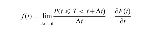
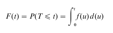
Suppose T is a continuous random variable indicating the duration of nonoccurrence of the first birth. Let f (t) be the probability density function of T, and F (t) the distribution function of T. As always the following relationships exist between these two quantities,

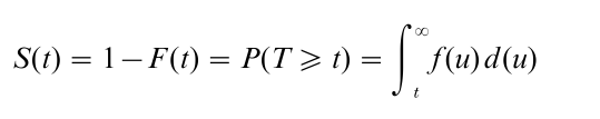
The survival probability or survival function, indicting the probability of nonoccurrence of an event until time t, is defined as

Another important concept is the hazard rate or hazard function, h(t), expressing the instantaneous risk of experiencing an event at T=t, given that the event did not occur before t. The hazard rate is defined as

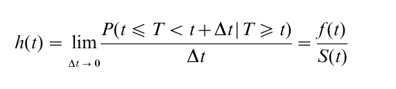
in which P(t≤T<t+∆t|T≥ t) indicates the probability that the event will occur during [t≤T<t+∆t], given that the event did not occur before t. The hazard rate is equal to the unconditional instantaneous probability of having an event at T= t, f (t), divided by the probability of not having an event before T=t, S(t). It should be noted that the hazard rate itself cannot be interpreted as a conditional probability. Although its value is always non-negative, it can take values greater than one. However, for small ∆t, the quantity h(t)∆t can be interpreted as the approximate conditional probability that the event will occur between t and t+∆t.

Above h(t) was defined as a function of f (t) and S(t). It is also possible to express S(t) and f (t) completely in terms of h(t), that is,

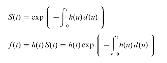
This shows that the functions f (t), F (t), S(t), and h(t) give mathematically equivalent specifications of the distribution of T.

4. Log-Linear Models For The Hazard Rate

When working within a continuous-time framework, the most appropriate method for regressing the time variable T on a set of covariates is through the hazard rate. This makes it straightforward to assess the effects of time-varying covariates—including the time dependence itself and time-covariate interactions—and to deal with censored observations. Censoring is a form of missing data that is explained in more detail below.

Let h(t|x_i) be the hazard rate at T=t for an individual with covariate vector xi. Since the hazard rate can take on values between 0 and infinity, most hazard models are based on a log transformation of the hazard rate, which yields a regression model of the form

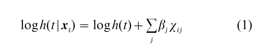
This hazard model is not only log-linear but also proportional. In proportional hazard models, the time-dependence is multiplicative (additive after taking logs) and independent of an individual’s covariate values. Below it will be shown how to specify nonproportional log-linear hazard models by including time-covariate interactions.

The various types of continuous-time log-linear hazard models are defined by the functional form that is chosen for the time dependence, that is, for the term log h(t). In Cox’s semi-parametric model, the time dependence is left unspecified (Cox 1972). Exponential models assume the hazard rate to be constant over time, while piecewise exponential model assume the hazard rate to be a step function of T, that is, constant within time periods. Other examples of parametric log-linear hazard models are Weibull, Gompertz and polynomial models.

As was demonstrated by several authors (Laird and Oliver 1981, Vermunt 1997, pp. 106–17), log-linear hazard models can also be defined as log-linear Poisson models, which are also known as log-rate models. Assume that we have—besides the event history information—two categorical covariates denoted by A and B. In addition, assume that the time axis is divided into a limited number of time-intervals in which the hazard rate is postulated to be constant. In the first birth example, this could be one-year intervals. The discretized time variable is denoted by Z. Let h_abz denote the constant hazard rate in the zth time interval for an individual with A=a and B=b. To see the similarity with standard log-linear models, it should be noted that the hazard rate, sometimes referred to as occurrence-exposure rate, can also be defined as h_abz =m_abz /E_abz. Here, m_abz denotes the expected number of occurrences of the event of interest and E_abz the total exposure time in cell (a, b, z).

Using the notation of hierarchical log-linear models, the saturated log-linear model for the hazard rate h_abz can now be written as

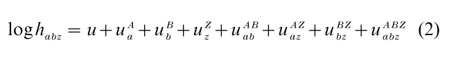
in which the u terms are log-linear parameters which are constrained in the usual way, for instance, by means of ANOVA-like restrictions. Note that this is a non-proportional model because of the presence of time-covariate interactions. Restricted variants of model described in equation (2) can be obtained by omitting some of the higher-order interaction terms. For example,

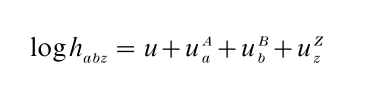
yields a model that is similar to the proportional log-linear hazard model described in equation (1). In addition, different types of hazard models can be obtained by the specification of the time-dependence. Setting the u_z ^Z terms equal to zero yields an exponential model. Unrestricted u_z ^Z parameters yield a piecewise exponential model. Other parametric models can be approximated by defining the u_z ^Z terms to be some function of Z. And finally, if there are as many time intervals as observed survival times and if the time dependence of the hazard rate is not restricted, one obtains a Cox regression model. Log-rate models can be estimated using standard programs for log-linear analysis using E_abz as a weight vector (Vermunt 1997, p. 112).

Unobserved heterogeneity or selectivity may bias the results obtained from the hazard models discussed so far in various ways. The best-known implication is the negative bias of the time dependence. Other implications are that covariate effects may be biased (underestimated) and that one may find spurious time-covariate interactions.

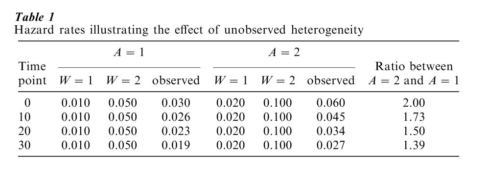
We will illustrate the effects of unobserved heterogeneity with a small example. Suppose that the population under study consists of two subgroups formed by the two levels of an observed covariate A, where for an average individual with A=2 the hazard rate is twice as high as for someone with A=1. In addition, assume that within each of the levels of A there is (unobserved) heterogeneity in the sense that there are two subgroups W=1 and W=2, where W=2 has a 5 times higher hazard rate than W=1. Table 1 shows the assumed hazard rates for each of the possible A–W combinations at four time points. As can be seen, the true hazard rates do not change over time given A and W. The reported hazard rates in the columns labeled ‘observed,’ which were obtained by setting up a simple life table, show what happens if we do not observe W. First, it can be seen that both for A=1 and A=2 the observed hazard rates decline over time while the true rates were time constant. This illustrates the fact that unobserved heterogeneity biases the estimated time dependence in a negative direction. Second, while the ratio between the hazard rates for A =2 and A=1 equals the true value 2.00 at t=0, it declines over time (see last column). Thus, when estimating a hazard model with these observed hazard rates, we will find a smaller effect of A than the true value of (log) 2.00. Third, in order to describe fully the pattern of observed hazard rates, we need to include a time-covariate interaction in the hazard model: the covariate effect changes (declines) over time or, equivalently, the (negative) time effect is smaller for A=1 than for A=2.

5. Censoring

A subject that always receives a great amount of attention in discussions on event history analysis is the problem of censoring. An observation is called censored if it is known that is did not experience the event of interest during some time, but it is not known when it experienced the event. In fact, censoring is a specific type of missing data. In the first-birth example, a censored case could be a woman which is 30 years of age at the time of interview (and has no follow-up interview) and does not have children. For such a woman, it is known that she did not have a child until age 30, but it is not known whether nor when she will have her first child. This is, actually, an example of what is called right censoring. Another type of censoring that is more difficult to deal with is left censoring. Left censoring means that we do not have information on the duration of nonoccurrence of the event before the start of the observation period.

As long as it can be assumed that the censoring mechanism is not related to the process under study, dealing with right censored observations in maximum likelihood estimation of the parameters of hazard models is straightforward. Let δ_i be a censoring indicator taking the value 0 if observation i is censored and 1 if it is not censored. The contribution of case i to the likelihood function that must be maximized when there are censored observations is

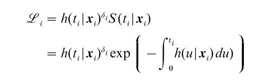
This likelihood function is, however, only valid if the censoring mechanism can be ignored for likelihood based inference. The presence of unobserved heterogeneity that is shared by the process of interest and the censoring process will lead to a violation of the assumption that censoring is ignorable.

6. Time-Varying Covariates

A strong point of hazard models is that one can use time-varying covariates. These are covariates that may change their value over time. Examples of interesting time-varying covariates in the first-birth example are a woman’s marital and work status. It should be noted that, in fact, the time variable and interactions between time and time-constant covariates are time-varying covariates as well.

The saturated log-rate model described in equation (2), contains both time effects and time-covariate interaction terms. Inclusion of ordinary time-varying covariates does not change the structure of this hazard model. The only implication of, for instance, covariate B being time varying rather than time constant is that in the computation of the matrix with exposure times E_abz it has to taken into account that individuals can switch from one level of B to another.

The presence of unobserved heterogeneity may seriously bias the effects of time-varying covariates. More precisely, the effects of time-varying covariates may be partially spurious as a result of the presence of unobserved risk factors influencing both the covariate process and the dependent process. An example of an association that may be partially spurious is the association between a woman’s labor participation and the first birth rate. In several studies, it has been found that women who are not employed have higher first birth rates than women who are employed. This association may, however, be partially the result of unobserved causes that work and fertility behavior have in common, such as certain gender role attitudes.

7. Multiple Risks

Thus far, only hazard rate models for situations in which there is only one destination state were considered. In many applications it may, however, prove necessary to distinguish between different types of events or risks. In the analysis of the first-union formation, for instance, it may be relevant to make a distinction between marriage and cohabitation. In the analysis of death rates, one may want to distinguish different causes of death. And in the analysis of the length of employment spells, it may be of interest to make a distinction between the events voluntary job change, involuntary job change, redundancy, and leaving the labor force.

The standard method for dealing with situations where—as a result of the fact that there is more than one possible destination state—individuals may experience different types of events is the use of a multiple-risk or competing-risk model. A multiplerisk variant of the hazard rate model described in equation (1) is

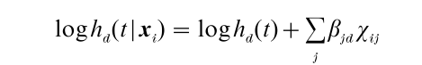
Here, the index d indicates the destination state or the type of event. As can be seen, the only thing that changes compared with the single type of event situation is that we have a separate set of time and covariate effects for each type of event.

Again the presence of unobserved heterogeneity may distort the results obtained from the hazard model. More precisely, if the different types of events have shared unmeasured risk factors, the results for each of the types of events have shared unmeasured risks factors, the results for each of the types of events is only valid under the observed hazard rates for the other risks. In fact, the resulting dependence among risks is comparable to what in the field of discrete choice modeling is known as the violation of the assumption of independence of irrelevant alternatives.

8. Repeatable Events And Other Types Of Multivariate Event Histories

Most events studied in social sciences are repeatable, and most event history data contains information on repeatable events for each individual. This is in contrast to biomedical research, where the event of greatest interest is death. Examples of repeatable events are job changes, having children, arrests, accidents, promotions, and residential moves.

Often events are not only repeatable but also of different types, that is, we have a multiple-state situation. When people can move through a sequence of states, events cannot only be characterized by their destination state, as in competing risks models, but they may also differ with respect to their origin state. An example is an individual’s employment history: an individual can move through the states of employment, unemployment, and out of the labor force. In that case, six different kinds of transitions can be distinguished which differ with regard to their origin and destination states. Of course, all types of transitions can occur more than once. Other examples are people’s union histories with the states living with parents, living alone, unmarried cohabitation, and married cohabitation, or people’s residential histories with different regions as states.

Hazard models for analyzing data on repeatable events and multiple-state data are special cases of the general family of multivariate hazard rate models. Another application of these multivariate hazard models is the simultaneous analysis of different life-course events. For instance, it can be of interest to investigate the relationships between women’s reproductive, relational, and employment careers, not only by means of the inclusion of time-varying covariates in the hazard model, but also by explicitly modeling their mutual interdependence.

Another application of multivariate hazard models is the analysis of dependent or clustered observations. Observations are clustered, or dependent, when there are observations from individuals belonging to the same group or when there are several similar observations per individual. Examples are the occupational careers of spouses, educational careers of brothers, child mortality of children in the same family, or in medical experiments, measures of the sense of sight of both eyes or measures of the presence of cancer cells in different parts of the body. In fact, data on repeatable events can also be classified under this type of multivariate event history data, since in that case there is more than one observation of the same type for each observational unit as well.

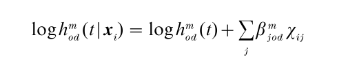
The hazard rate model can easily be generalized to situations in which there are several origin and destination states and in which there may be more than one event per observational unit. The only thing that changes is that we need indices for the origin state (o), the destination state (d ), and the rank number of the event (m). A log-linear hazard rate model for such a situation is

The different types of multivariate event history data have in common that there are dependencies among the observed survival times. These dependencies may take several forms: the occurrence of one event may influence the occurrence of another event; events may be dependent as a result of common antecedents; and survival times may be correlated because they are the result of the same causal process, with the same antecedents and the same parameters determining the occurrence or nonoccurrence of an event. If these common risk factors are not observed, the assumption of statistical independence of observation is violated, which may seriously distort the results.

9. Model-Based Approaches To Unobserved Heterogeneity

As described in the previous sections, unobserved heterogeneity may have different types of consequences in hazard modeling. The best-known phenomenon is the downwards bias of the duration dependence. In addition, it may bias covariate effects, time-covariate interactions, and effects of time-varying covariates. Other possible consequences are dependent censoring, dependent competing risks, and dependent observations. This section presents two types of methods that have been proposed for correcting for unobserved heterogeneity: random-effects and fixed-effects methods.

9.1 Random-Effects Approach

The random-effects approach is based on the introduction of a time-constant latent covariate in the hazard model (Vaupel et al. 1979). This unobserved variable is assumed to have a multiplicative and proportional effect on the hazard rate, i.e.,

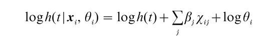
Here, θ_i denotes the value of the latent variable for subject i. In the parametric random-effects approach, the latent variable is postulated to have a particular distributional form. The amount of unobserved heterogeneity is determined by the size of the standard deviation of this distribution: The larger the standard deviation of θ_i or log θ_i, the more unobserved heterogeneity there is. Vaupel et al. (1979) proposed using a gamma distribution for θ_i, with a mean of 1 and a variance of 1/γ, where γ is the unknown parameter to be estimated. Another option would be to assume log θ_i to come from a normal distribution with mean zero and standard deviation σ.

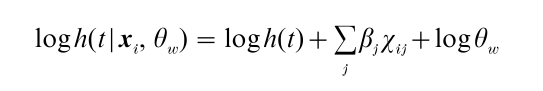
Heckman and Singer (1982) demonstrated that the results obtained from continuous-time hazard models can be sensitive to the choice of the functional form of the distribution of the random effect. Therefore, they advocated using a nonparametric characterization of this distribution by means of a finite set of mass points whose number, locations, and weights are empirically determined. The nonparametric random-effects model proposed by Heckman and Singer is, actually, a latent class or finite mixture model. As in latent class analysis, the population is assumed to be composed of a finite number of exhaustive and mutually exclusive groups formed by the categories of an unobserved variable. Suppose W is a categorical latent variable with W * categories, and w is a particular value of W. The model of Heckman and Singer can be formulated as follows:

Here, θ_w denotes the (multiplicative) effect on the hazard rate for latent class w. The contribution of the ith subject to the likelihood function in the case of a single non-repeatable event is

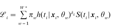
where π_w is the proportion of the population belonging to latent class w. In the terminology used by Heckman and Singer (1982), the number of latent classes (W *), the latent proportions (π_w), and the effects of W(θ_w) are called the number of mass points, the weights, and the mass points locations, respectively.

The most important drawback of the parametric and nonparametric random-effects approaches to unobserved heterogeneity is that the latent variable is assumed to be independent of the observed covariates. This is, in fact, in contradiction to the omitted variables argument that is often used to motivate the use of these types of mixture models. If one assumes that particular important variables are not included in the model, it is usually implausible to assume that they are completely unrelated to the observed factors. In other words, by assuming independence among unobserved and observed factors, the omitted variable bias, or selection bias, will generally remain (Chamberlain 1985, Yamaguchi 1986, 1991, p.132). To overcome the limitations of the standard randomeffects approaches, Vermunt (1997) proposed a more general nonparametric latent variable approach to unobserved heterogeneity. It differs from Heckman and Singer’s method in that different types of specifications can be used for the joint distribution of the observed covariates, the unobserved covariates, and the initial state. This makes it possible to specify hazard models in which the unobserved factors are related to the observed covariates and to the initial state.

9.2 Fixed-Effects Approach

A second method for dealing with unobserved heterogeneity involves adding cluster-specific effects, or incidental parameters, to the model (Chamberlain 1985, Yamaguchi 1986). In fact, a categorical variable is included in the hazard model indicating to which cluster a particular observation belongs: observations belonging to the same cluster have the same value for this ‘observed’ variable while observations belonging to different clusters have different values. This approach to unobserved heterogeneity, which is called the fixed-effects approach, can only be applied with multivariate survival data, that is, when there is more than one observation for the largest part of the observational units. Note that actually the unobserved heterogeneity is transformed into a form of observed heterogeneity capturing the similarity among observations belonging to the same cluster.

The advantage of using fixed-effects methods to correct for unobserved heterogeneity is that they circumvent two objections against random-effects methods presented above: No functional form needs to be specified for the distribution of the unobserved heterogeneity and the unobserved heterogeneity is automatically related to both the initial state and the time-constant covariates.

The major limitation of the fixed-effects approach is that since each cluster has its own incidental parameter, no parameter estimates can be obtained for the effects of covariates having the same value for the different observations belonging to the same cluster: Only the effects of observation-specific or of time-varying covariates can be estimated. Another problem is that the incidental parameters cannot be estimated consistently, since by definition they are based on a limited number of observations regardless of the sample size. This inconsistency may be carried over to the other parameters if the parameters are estimated by means of maximum likelihood (Yamaguchi 1986).

Bibliography:

1. Allison P D 1984 Event History Analysis: Regression for Longitudinal Event Data. Sage, London
2. Blossfeld H P, Rohwer G 1995 Techniques of Event History Modeling. Lawrence Erlbaum, Mahwah, NJ
3. Chamberlain G 1985 Heterogeneity, omitted variable bias, duration dependence. In: Heckman J J, Singer B (eds.) Longitudinal Analysis of Labor Market Data. Cambridge University Press, Cambridge, UK
4. Cox D R 1972 Regression models and life tables. Journal of the Royal Statistical Society B 34: 187–203
5. Heckman J J, Singer B 1982 Population heterogeneity in demographic models. In: Land K, Rogers A (eds.) Multidimensional Mathematical Demography. Academic Press, New York
6. Laird N, Oliver D 1981 Covariance analysis of censored survival data using log-linear analysis techniques. Journal of the American Statistical Association 76: 231–40
7. Lancaster T 1990 The Economic Analysis of Transition Data. Cambridge University Press, Cambridge, UK
8. Tuma N B, Hannan M T 1984 Social Dynamics: Models and Methods. Academic Press, New York
9. Vaupel J W, Manton K G, Stallard E 1979 The impact of heterogeneity in individual frailty on the dynamics of mortality. Demography 16: 439–54
10. Vermunt J K 1997 Log-linear models for event history histories. Advanced Quantitative Techniques in the Social Sciences Series. Vol. 8. Sage, Thousand Oaks, CA
11. Yamaguchi K 1986 Alternative approaches to unobserved heterogeneity in the analysis of repeatable events. In: Tuma N B (ed.) Sociological Methodology 1986. 213–49. American Sociological Association, Washington, DC
12. Yamaguchi K 1991 Event history analysis. Applied Social Research Methods, Vol. 28. Sage, Newbury Park, CA