Correspondence Analysis Research Paper

1. Row And Column Profiles

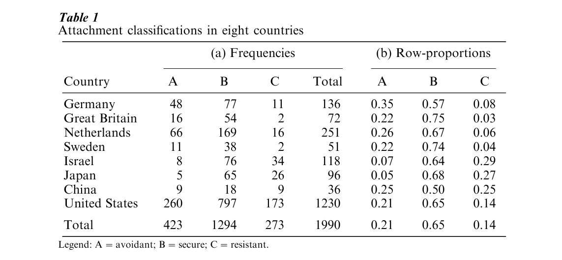
As an illustration consider the eight discrete distributions in Table 1(a) taken from van Ijzendoorn and Kroonenberg (1988). Several studies using the Strange Situation paradigm (Ainsworth et al. 1978) in various countries seemed to show marked cross-cultural differences in distributions of attachment classifications. Most of the studies used a classic three-fold attachment classification into Avoidant (A), Secure (B), and Resistant (C). These three types characterize the enduring socio-emotional bond between child and regular care-giver. To examine the cross-cultural heterogeneity more closely, the authors selected 32 samples from eight countries, representing 1,990 Strange Situation classifications, which have been aggregated in Table 1 to the level of countries. To study similarities and differences of distributions regardless of sample size, it is necessary to divide frequencies by their row total (see Table 1(b)). A row of proportions is called a row profile; analogously, a column profile is formed by dividing the cell frequencies in a column by the column total. The natural comparison standard to assess a row profile against is the marginal profile of the columns, that is, each of the column totals divided by n, the grand total. Similarly, column profiles are first compared with the marginal profile of the rows, that is, each of the row totals divided by n. From the row profiles it is immediately clear that Germany has a relatively large proportion of Avoidant, for example, Great Britain and Sweden have an overrepresentation of Secure and an under-representation of Resistant, while Israel, Japan, and China have an overrepresentation of Resistant.

The aim of CA is to assess similarities and differences of row profiles (and/or column profiles), not only with respect to their marginal profile, but also amongst each other, by constructing a parsimonious approximation of the cell frequencies. The approximation consists of decomposing the correspondence table into one or more components, which through graphical display allows a deeper insight into the original categories by suggesting specific groupings, orderings, or more complicated arrangements.

2. Deviations From Independence

The decomposition of CA has two major parts: one consisting of a multiplicative combination of row and column proportions, the usual form used in studying statistical independence, the other consisting of row– column interaction effects. To be more explicit, the following notation is introduced.

The frequency in cell (i, j ) of the contingency table is denoted by n_ij, where the categories of the row variable A have range i=1, …, I and the categories of the column variable B have range j=1, …, I, and the categories of the column variable B have range j=1, …, J. Row totals are defined as n_i+ = Σ_jn_ij and column totals as n_+j = Σ_in_ij. We also have the grand total n₊₊ = Σ_in_i+ = Σ_jn_+j, frequently denoted simply by n. To keep the results invariant under changes in sample size, CA works with the quantities p_ij = n_ij/n, each of which is the (estimated) probability mass in the cell (i, j) of the bivariate distribution of A and B, r_i =n_i+/ n, the relative mass of row profile i, and c_j= n_+j /n, the relative mass of column profile j. The CA decomposition is based on the tautologous identity

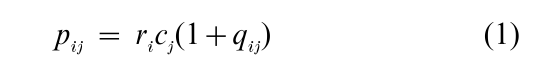
where the quantities q_ij are defined as q_ij =( p_ij-r_ic_j)/(r_ic_i). The q_ij are standardized deviations from independence: if the two variables A and B are independent, we have p_ij = r_ic_j and every q_ij would vanish. Dependences between A and B show up specifically in the q_ij: categories i and j are more strongly associated than expected under independence when q_ij > 0, and less strongly when q_ij >0. Spatial and graphical representations that result from CA are representations of the deviations [q_ij], not of the data [ p_ij] themselves.

3. Basic Geometric Model

In the CA model each row profile initially is a point a_i in a subspace of dimensionality J-1, with coordinates a_ij =n_ij /n_i+. Analogously, each column profile is a point b_j with coordinates b_ij= n_ij /n_+j in another subspace, of dimensionality I-1. The total spread of the points in space is measured by their inertia J, a concept from physics defined as (for the row points)

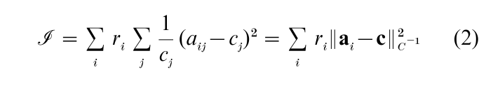
where c is the point with coordinates cj that represents the marginal profile of the columns. The function ||·||_C−1 defined implicitly in Eqn. (2) is a Euclidean norm with weights 1/c_j. It downweights column differences associated with large column mass, because large frequencies tend to be less reliable. There is a parallel expression of inertia for column points, which can be shown to yield the same numerical value of J. In both cases, large overall differences among the distributions will lead to a spread-out configuration of points with large J , while small overall differences will correspond to a tight concentration of points around their center of gravity, with small J.

Dividing the usual chi-squared statistic by n, so that lack of homogeneity (or independence) is measured regardless of sample size, we have the equality

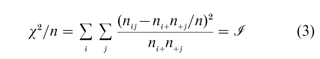
In statistics, χ²/n is known as Pearson’s mean square contingency. The r elation in Eqn. (3) between the chi- squared statistic χ² and the weighted sum of squared distances towards the center of gravity J defined in Eqn. (2) is the reason that one speaks of heterogeneity being measured in the chi-squared metric ||·||_{C−1 .}

Mutual distances between row profiles are determined in the same chi-squared metric, and hence called chi-squared distances. For two profiles i and k we have

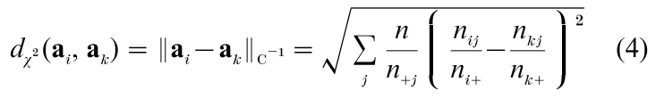
with again an analogous expression for the column points. In Eqn. (4) columns with small marginal frequency are seen to contribute more to overall lack of similarity than columns with large marginal frequency. For an exhaustive treatment of the geometry of CA, see Benzecri (1992, pt. I).

4. Weighted Least Squares Approximation

Low-dimensional CA approximations of the full-dimensional model are obtained by least squares, where each cell is weighted by the product of the row and column masses (see Andersen 1990). The least squares solution consists of two sets of standardized coordinates, z_it(A) and z_jt(B), where t indexes the components, with t having range t=1, …, min (I-1, J-1). The components are ordered by the size of a third set of quantities σ_t, called singular values. Stan dardized coordinates zit(A) have the property Σ_ir_iz²_it(A)=1; analogously, for z_jt(B) we have Σ_jc_jz_jt²(B) =1. Also, the coordinates are in deviation from their weighted mean and uncorrelated across different values of t. The singular values σ_t indicate the relative importance of component t in the approximation of [q_ij]. Practical CA solutions are obtained by dropping components associated with small singular values.

Graphical displays are based upon a mapping from a_i to y_i(A), a model point with principal coordinates defined as y_it(A) =σ_tz_it(A), with t =1, …, T (some chosen dimensionality). Principal coordinates for column points are y_jt(B) =σ_tz_jt(B). For maximal dimensionality T*=min(I-1, J-1) it can be shown that

i.e., Euclidean distances among model points are equal to chi-squared distances among profile points. In approximations with T<T* the former are always smaller than latter (see Meulman 1982).

5. Some Important Additional Concepts

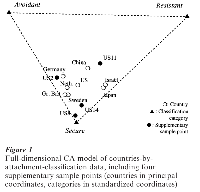
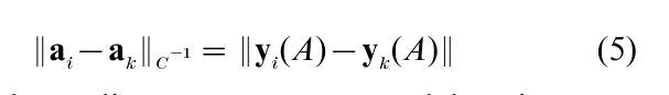
The CA solution for the attachment data is shown in Fig. 1, in which the row points are plotted as open circles. Since in this example we have T*=2, the model exactly reproduces the data ( χ²=102.42 with df4, J=0.051). Approximation in T=1 implies projecting all points on the horizontal axis, which here accounts for 86 percent of the inertia (see Fig. 2). With the US and China forming the center, the largest contrast in both solutions is between the Western European countries vs. Israel and Japan, while Fig. 1 shows a second contrast between China and Germany versus Great Britain and Sweden related to deviations in their Secure classifications.

5.1 Transition Formulas

Row points and column points reside in two different but intimately related spaces. Their coordinates are connected by the equations

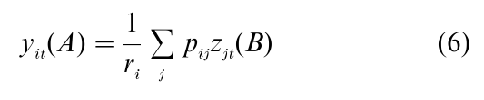
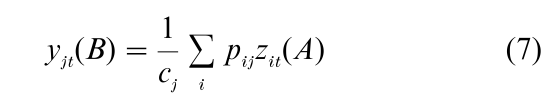
These equations are called transition formulas, since they show how the principal coordinates, e.g., y_it(A), of one set of points can be obtained from the standardized coordinates, e.g., z_jt(B), of the other set of points: by weighted averaging with the data as coefficients. If the correspondence table is binary, principal coordinates are plain averages of standardized coordinates, and CA becomes equivalent to the method of reciprocal averages, which has firm roots in psychometrics (Horst 1935, Guttman 1941), with continued research under the name dual scaling (Nishisato 1994).

5.2 Joint Plot And Coherent Normalization

In Fig. 1 the country points are plotted in principal coordinates, so that their Euclidean distances are equal to the chi-squared distance of Eqn. (5). The distances between the country markings along the line in Fig. 2 approximate these chi-squared distances rather closely. The plots also show the three attachment classes in standardized coordinates. Super-position of row and column points forms a joint plot, also called a ‘biplot,’ which is easily interpretable due to the transition formulas. For example, Germany is located relatively close to Avoidant, because its location is a weighted average of the three attachment points, weighted with [0.35, 0.57, 0.08] rather than with the average profile [0.21, 0.65, 0.14], which forms the center of the plot. It is also possible to (re)scale the coordinates so as to make the two clouds of points more evenly mixed, but this has to be done with some care (Heiser and Meulman 1983). Rescaling is coherent if we choose points x_i(A) and x_j(B ) with coordinates x_it(A) = σ^α_t z_it(A) and x_jt(B) =σ_t^1–a z_it(B) for any α, because it remains true that x_i(A)^Tx_j(B)=q_ij. But it should be noted that we no longer approximate chi-squared distance unless α=0 or α=1.

5.3 Supplementary Points

It can be useful to add new profiles to an existing joint plot. These supplementary points are easily obtained if scaling is chosen as α=0 or α=1, since then Eqns. (6) or (7) can be used to find coordinates. In Fig. 1, points were added for four divergent individual US studies, showing that there is at least as much variation within the US as between countries. While US2 closely resembles the total German group, US11 is much more like China, for example.

6. Extensions And Applications

The case of more than two variables, called multiple CA, was pioneered by Guttman (1941). Under the name ‘homogeneity analysis,’ Gifi (1990) generalized Guttman’s technique to ordinal data, and introduced extensions based on partitioning of variables. Green-acre (1984) and Lebart et al. (1984) bridged the gap between the early French work and the international literature. The edited volume of Greenacre and Blasius (1994) contains social science applications, versions of CA with various constraints, and versions that achieve clustering of categories.

Bibliography:

1. Ainsworth M D S, Blehar M C, Waters E, Wall S 1978 Patterns of Attachment, a Psychological Study of the Strange Situation. Erlbaum, Hillsdale, NJ
2. Andersen E B 1990 The Statistical Analysis of Categorical Data. Springer, Berlin
3. Benzecri J-P 1992 Correspondence Analysis Handbook. Dekker, New York
4. Gifi A 1990 Nonlinear Multivariate Analysis. Wiley, New York
5. Greenacre M J 1984 Theory and Applications of Correspondence Analysis. Academic, London
6. Greenacre M, Blasius J (eds.) 1994 Correspondence Analysis in the Social Sciences. Academic, London
7. Guttman L 1941 The quantification of a class of attributes: A theory and method of scale contribution. In: Horst P et al. (eds.) The Prediction of Personal Adjustment. Social Science Research Council, New York, pp. 319–48
8. Heiser W J, Meulman J J 1983 Analyzing rectangular tables with joint and constrained multidimensional scaling. Journal of Econometrics 22: 139–67
9. Horst P 1935 Measuring complex attitudes. Journal of Social Psychology 6: 369–74
10. Lebart L, Morineau A, Warwick K M 1984 Multivariate Descriptive Statistical Analysis: Correspondence Analysis and Related Techniques for Large Matrices. Wiley, New York
11. Meulman J J 1982 Homogeneity Analysis of Incomplete Data. DSWO, Leiden, The Netherlands
12. Nishisato S 1994 Elements of Dual Scaling: An Introduction to Practical Data Analysis. Erlbaum, IIillsdale, NJ
13. van Ijzendoorn M H, Kroonenberg P M 1988 Cross-cultural patterns of attachment: a meta-analysis of the strange situation. Child Development 59: 147–56