Optimal Control Theory Research Paper

It turns out that in solving an optimal control problem, it is useful to add a new set of variables, called co-state variables: for each state variable, one assigns a corresponding co-state variable. In economics, the co-state variables are often called shadow prices, because each co-state variable is an indicator of the worth of the associated state variable to the decision maker. With this additional set of variables, one can formulate an elegant set of necessary conditions, called the maximum principle, which is extremely useful in constructing the solution for the optimal control problem, and which, as a bonus, provides deep insight into the nature of the solution.

1. The Maximum Principle

We now define a simple optimal control problem and state the maximum principle for it. Let t denote time. Let s(t) = (s₁(t), s₂(t), … , s_n(t)) be the vector of n state variables, and c(t) = (c₁(t), c₂(t), … , c_m(t)) be the vector of m control variables. (m can be greater than, equal to, or less than n.) The transition equations are given by

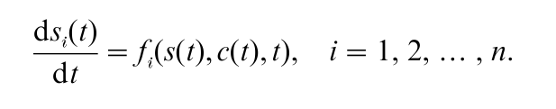
and the initial values of the state variables are s_i(0) = s_i0, i = 1, 2, … , n. The terminal time T is fixed in this simple problem. The decision maker must find the time path of c(t) to maximize the sum of (a) the value of integral of the flow of net benefit, with the benefit at time t being denoted by u(s(t), c(t), t), and (b) the value of the terminal stocks, denoted by φ(s(T ), T ):

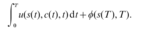
 (The functions u( ), φ( ), and f_i( ) are exogenously specified.) At each time t, the values that c(t) can take on are restricted to lie in a certain set A.

For each state variables s_i, one introduces a corresponding co-state variable π_i. Let π(t) = (π₁(t), π₂(t), … , π_n(t)). The co-state variables must satisfy certain conditions, as set out below, and their optimal values must be determined as part of the solution of the problem. A key step in solving an optimal control problem is the construction of a function called the Hamiltonian, denoted as H(s(t), c(t), π(t), t), and defined as

The maximum principle states that an optimal solution to the above problem is a triplet (s(t), c(t), π(t)) that satisfies the following conditions.

(a) c(t) maximizes H(s(t), c(t), π(t), t) for given s(t), π(t), and t, over the set A. (This is a very attractive property, because the Hamiltonian can be interpreted as the sum of the current benefit and an indicator of future benefits arising from current actions, as reflected in the value of the rates of change of the state variables that are influenced by the control variables.)

(b) The co-state variables and the state variables are related by the equations

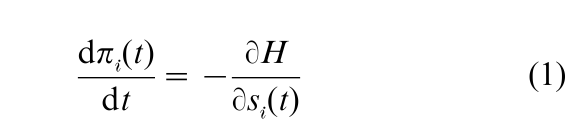
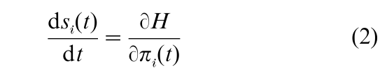
Note that Eqn. (1) has the following appealing interpretation. The co-state variable π_i being the shadow price of the state variable s_i, the left-hand side of (1) may be thought of as the capital gain (the increase in the value of that asset). The optimal level of asset holding must be such that the sum of (a) the marginal contribution of that asset, ϭH/ϭs_i(t), and (b) the capital gain term, is equal to zero.

(c) 2n boundary conditions must be met, namely, s_i(0) = s_i0, i = 1, 2, … , n, and

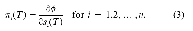
The conditions given by (3) are also called the transversality conditions. They say that at the terminal time T there must be an equality between π_i(T ) (the ‘internal worth’ of the stock i) and its ‘external worth’ at the margin (recall that the function φ( ) is externally specified).

The optimal time path of the control variables can be represented either in the open-loop form, i.e., each c_i(t) is expressed as a function of the time, having as parameters the initial conditions s_0i= (i = 1, 2, … , n), or in the closed-loop form, or feedback form, i.e., an optimal rule which determines c(t) using only the knowledge of the concurrent values of the state variables, and of t.

There are more complicated optimal control problems, which may involve several initial or terminal constraints on the state variables, or the optimal choice of the terminal time T (no longer fixed), or of the initial time (for example, at what time a mining firm should abandon a mine, a researcher should drop a research project, or a city should start building an airport). These problems give rise to a complex set of transversality conditions; see Leonard and Long (1992) for a useful tabulation.

2. Connections With The Calculus Of Variations And Dynamic Programming

Optimal control theory has its origin in the classical calculus of variations, which concerns essentially the same type of optimization problems over time. However, with the maximum principle, developed by Pontryagin and his associates (see Pontryagin et al. 1962), the class of problems that optimal control theory can deal with is much more general than the class solvable by the calculus of variations.

Optimal control theory is formulated in continuous time, though there is also a discrete time version of the maximum principle; see Leonard and Long (1992). In discrete time, the most commonly used optimization technique is dynamic programming, developed by Bellman (1957), using a recursive method based on the principle of optimality. Bellman’s principle of optimality can also be formulated in continuous time, leading to the Hamilton–Jacobi–Bellman equation (or HJB equation for short), which is closely related to Pontryagin’s maximum principle, and is often used to provide a heuristic proof of that principle (see Arrow and Kurz 1970). Such a heuristic proof reveals that the shadow price (i.e., the co-state variable) of a given state variable is in fact the derivative of the value function (obtained in solving the HJB equation) with respect to that state variable, thus justifying the name shadow price. This approach yields equations that are in agreement with (b) in the preceding section.

3. Applications Of Optimal Control Theory To Economics, Finance, And Management Sciences

Economists initially made use of optimal control theory primarily to address the problem of optimal capital accumulation and optimal management of natural resources and the environment (Arrow and Kurz 1970, Hadley and Kemp 1971, Pitchford and Turnovsky 1977, Kemp and Long 1980). Optimal control theory has been used to study a variety of topics, such as macroeconomic impacts of fiscal policies in a well-functioning market economy (for example, the effect of a temporary increase in government spending on private consumption and investment), optimal consumption planning by an individual (for example, Becker and Murphy (1988) addressed the question of rational addiction: if you know that your current level of consumption of a drug will determine your degree of addiction which in turn will increase your future demand for it, how should you determine your time path of consumption of the drug, knowing the consequence of addiction?).

In management science, optimal control theory has been applied to management problems such as the optimal holding of inventories, the optimal time path of advertising (e.g., under what conditions would it be optimal to vary the intensity of advertising over the product cycle), the optimal maintenance and sale age for a machine subject to failure, and so on. In finance, theories of optimal portfolio adjustments over time, and theories on the pricing of financial options, have been developed using optimal control methods, in a stochastic setting. (See Malliaris and Brock 1982).

It is important to note that while the variable t often stands for time, and the objective function is often an integral over a time interval, it is not necessary to restrict the theory to that interpretation. In fact, in some important applications of optimal control theory to economics, t has been interpreted as an index of the type of an individual in a model where there is a continuum of types.

4. Extensions Of Optimal Control Theory

There are two important extensions of optimal control theory. The first extension consists of allowing for uncertainty in the transition equations, leading to the development of stochastic optimal control theory. The second extension is to allow for strategic interactions among decision makers who pursue different objectives, or who have diametrically opposed interests. The body of literature which deals with this extension is called differential game theory.

4.1 Stochastic Optimal Control Theory

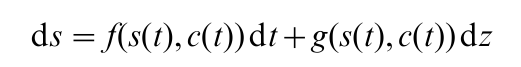
A typical transition equation in stochastic optimal control theory is

where dz represents an increment of a stochastic process z called the Wiener process. In this equation, f(s(t), c(t)) represents the expected rate of change in the state variable s, the term dz represents a random disturbance in the external environment, and g(s(t), c(t)) indicates that the effect of that disturbance on the evolution of the state variable may depend on the values taken by the control variable and the state variable.

In some contexts, it is more appropriate to consider random disturbances that occur only rarely, but that may have great impacts when they occur, for example, an earthquake, a currency crisis, or a discovery of an entirely new production technique. To deal with such discrete events, the Poisson process (also called jump process) is used instead of the Wiener process, which is suitable for continuous random variations.

In finding a solution of a stochastic optimal control problem, one makes use of a stochastic version of the Hamilton–Jacobi–Bellman equation. Sometimes it is possible to provide an explicit solution in the feedback form. For example, some adjustment rules for portfolios of financial assets can be derived. Another interesting application of stochastic optimal control is the problem of determining the optimal time to switch from one regime to another. This is often referred to as the optimal stopping problem. One asks, for example, when one should exercise a call option (stop waiting for a further increase in price), or when to start setting up a factory in a foreign country (stop waiting for a further favorable movement of the exchange rate).

4.2 Differential Games

An example of a differential game can be given involving a transboundary fishery: two nations have access to a common fish stock. Each nation knows that the other nation’s harvesting strategy will have an impact on the fish stock. If the two nations do not cooperate, they are said to be players in a noncooperative game. Each nation would be solving an optimal control problem, taking as given the strategy of the other nation. In trying to predict the outcome of such non-cooperative games, theorists have formulated various concepts of equilibrium. A Nash equilibrium of a differential game is a pair of strategies, one for each player, such that each player’s strategy is the best course of action (i.e., it solves the player’s optimal control problem), given the strategy of the other player.

The nature of the solution depends on the set of strategies available to the players. If one assumes that, given the initial conditions, players can only choose control variables as functions of time (and not as functions of the concurrent values of the state variables), then the equilibrium is called an open-loop Nash equilibrium. On the other hand, if players must choose strategies that specify the values to be taken by the control variables at any time as functions of the concurrent values of the state variables, and possibly of time, then the equilibrium is said to be a feedback Nash equilibrium. A refinement of the feedback Nash equilibrium requires that at any point of time, and given any situation the system may reach, the rule chosen by each player must remain optimal for that player, given that other players do not change their rules. This property is called subgame perfectness. A feedback Nash equilibrium that satisfies the subgame perfectness property is called a Markov Perfect Nash equilibrium.

Both deterministic and stochastic differential games have been applied to problems in economics and management science. Examples include games of transboundary fishery, advertising games, innovation games, and so on (see Clemhout and Wan 1994, and Dockner et al. 2000).

5. Conclusions And Future Directions

Optimal control theory has become a standard tool in economics and management science. It has facilitated the solution of many dynamic economic models, and helped to provide a great deal of insight into rational behavior and interactions in a temporal context. Several unsolved problems are currently attracting research interests. Among these are (a) finding Markov-perfect equilibria for general dynamic games with a hierarchical structure (some players have priority of moves), and (b) the search for optimal policy rules that are dynamically consistent in an environment where economic agents are rational forecasters.

Bibliography:

1. Arrow K J, Kurz M 1970 Public Investment, the Rate of Return, and Optimal Fiscal Policy. Johns Hopkins University Press, Baltimore
2. Becker G S, Murphy K M 1988 A theory of rational addiction. Journal of Political Economy 96(4): 675–700
3. Bellman R 1957 Dynamic Programming. Princeton University Press, Princeton, New Jersey
4. Clemhout S, Wan H Jr. 1994 Differential games: Economic applications. In: Aumann R, Hart S (eds.) Handbook of Game Theory, with Economic Applications. North-Holland, Amsterdam, Chap. 23
5. Dockner E, Jorgensen S, Long N V, Sorger G 2000 Differential Games in Economics and Management Science. Cambridge University Press, Cambridge, UK
6. Hadley G, Kemp M C 1971 Variational Methods in Economics. North-Holland, Amsterdam
7. Kemp M C, Long N V 1980 Exhaustible Resources, Optimality, and Trade. North-Holland, Amsterdam
8. Leonard D, Long N V 1992 Optimal Control Theory and Static Optimization in Economics. Cambridge University Press, Cambridge, UK
9. Malliaris A G, Brock W A 1982 Stochastic Methods in Economics and Finance. North-Holland, Amsterdam
10. Pitchford J D, Turnovsky S J 1977 Applications of Control Theory to Economic Analysis. North-Holland, Amsterdam Pontryagin L S, Boltyanski V G, Gamkrelidze R V, Mishchenko
11. E F 1962 The Mathematical Theory of Optimal Processes. Wiley, New York