Event History Analysis Applications Research Paper

1. Examples Of Continuous-Time, Discrete-State Processes

Event history analysis is the study of processes that are characterized in the following general way: (a) there is a collection of units (which may be individuals, organizations, societies, etc.), each moving among a finite (usually small) number of states; (b) these changes (or events) may occur at any point in time (i.e., they are not restricted to predetermined points in time); and (c) there are time-constant and/or time varying factors influencing the timing of events. Examples are workers who move between unemployment and employment; men and women who enter into consensual unions or marriages; companies that are founded or closed down; governments that break down; people who are mobile between different regions or nation states; consumers who switch from one brand to another; prisoners who are released and commit another crime; people, who show certain types of verbal and nonverbal behaviors in social interactions; students who drop out of school; incidences of racial and ethnic confrontation, protest, riot and attack; people who show signs of psychoses or neuroses; patients who switch between the states ‘healthy’ and ‘diseased,’ and so on. In event history analysis, the central characteristics of the underlying stochastic process is mirrored in the specific way theoretical and mathematical models are built, data are collected, and the estimation and evaluation of models is done.

2. Different Observation Plans

In event history analysis the special importance of broader research design issues has been stressed. In particular, different observation plans have been used to collect information on the continuous-time, discrete-state substantive process. These various schemes produce different types of data that constrain the statistical analysis in different ways: cross-sectional data, event count data, event sequence data, panel data, and event history data.

The cross-sectional observation design is still the most common form of data collection in many fields. A cross-sectional sample is only a ‘snapshot’ taken on the continuous-time, discrete-state substantive process (e.g., the jobs of people at the time of the interview). Event history analysis has shown that one must be very cautious in drawing inferences about explanatory variables on the basis of such data because, implicitly or explicitly, social researchers have to assume that the process under study is in some kind of equilibrium. Equilibrium means that the state probabilities are fairly trendless and the relationships among the variables are quite stable over time. Therefore, an equilibrium of the process requires that the inflows to and the outflows from each of the discrete states be equal over time to a large extent. This is a strong assumption that is not very often justified in the social and behavioral sciences (see Blossfeld and Rohwer 1995).

A comparatively rare type of data on changes of the process are event count data (Andersen et al. 1993). They record the number of different types of events for each unit in an interval (e.g., the number of racial and ethnic confrontations, protests, riots or attacks in a period of 10 years). Event sequence data provide even more information. They record the sequence of specific states occupied by each unit over time. The temporal data most often available to the scientist are panel data. They provide information on the same units of analysis at a series of discrete points in time. In other words, there is only information on the states of the units at predetermined survey points and the course of the process between the survey points remains unknown. Panel data certainly contain more information than cross-sectional data, but involve well-known distortions created by the method itself (e.g., panel bias, attrition of sample). In addition, causal inferences based on panel approaches are much more complicated than has been generally acknowledged (Blossfeld and Rohwer 1995). With regard to the continuous-time, discrete-state substantive process, panel analysis is particularly sensitive to the length of the time intervals between the waves relative to the speed of the process. They can be too short, so that too few state transitions will be observed, or too long, so that it is difficult to establish a time-order between the events.

The event oriented observation design records the complete sequence of states occupied by each unit and the timing of changes among these states. For example, an event history of job mobility consists of more or less detailed information about each of the jobs and the exact beginning and ending dates of each job. Thus, this is the most complete information one can get on the continuous-time, discrete-state substantive process. Such event history data are often collected retrospectively with life history studies. Life history studies are normally cheaper than panel studies and have the advantage that they code the data into one framework of codes and meaning. But retrospective studies also suffer from several limitations (see Blossfeld and Rohwer 1995). In particular, data concerning motivational, attitudinal, cognitive, or affective states are difficult (or even impossible) to collect retrospectively because the respondents can hardly recall the timing of changes in these states accurately. Also the retrospective collection of behavioral data has a high potential for bias because of its strong reliance on autobiographic memory. To reduce these problems of data collection, modern panel studies (e.g., the Panel Study of Income Dynamics (PSID) in the USA, the British Household and Panel Survey (BHPS) in the UK, or the Sozio-oekonomisches Panel (SOEP) in Germany) use a mixed design which provides traditional panel data and retrospectively collects event history data for the period before the first panel wave and between the successive panel waves.

3. Event History Analysis

Event history analysis, originally developed as independent applications of mathematical probability theory in demography (e.g., the classical life table analysis and the product-limit estimator of Kaplan and Meier (1958), reliability engineering, and biostatistics (e.g., the path-breaking semiparametric regression model for survival data of David Cox (1972) has gained increasing importance in the social and behavioral sciences (see Tuma and Hannan 1984, Blossfeld et al. 1989, Lancaster 1990, Andersen et al. 1993, Blossfeld and Rohwer 1995) since the early 80s. Due to the development and application of these methods in various disciplines, the terminology is normally not easily accessible to the user. Central definitions are therefore given first.

3.1 Basic Terminology

Event history analysis studies transitions across a set of discrete states, including the length of time intervals between entry to and exit from specific states. The basic analytical framework is a state space and a time axis. The choice of the time axis or clock (e.g., age, experience, marriage duration, etc.) used in the analysis must be based on theoretical considerations and affects the statistical model. Dependent on practical and theoretical reasons, there are event history methods using a discrete (Yamaguchi 1991, Vermunt 1997) or continuous time axis (Tuma and Hannan 1984, Blossfeld et al. 1989, Courgeau and Lelievre 1992, Blossfeld and Rohwer 1995). Discrete-time event history models are, however, special cases of continuous-time models and are therefore not further discussed here. An episode, spell, waiting time, or duration—terms that are used interchangeably in the literature—is the time span a unit of analysis (e.g., an individual) spends in a specific state. The states are discrete and usually small in number. The definition of a set of possible states, called the state space, is also dependent on substantive considerations. Thus, a careful, theoretically driven choice of the time axis and design of state space are crucial because they are often serious sources of mis-specification.

The most restricted event history model is based on a process with only a single episode and two states (an origin state j and a destination state k). An example may be the duration of first marriage until the end of the marriage, for whatever reason (separation, divorce, death). In the single episode case each unit of analysis that entered into the origin state is represented by one episode. Event history models are called multistate models, if more than one destination state exists. Models for the special case with a single origin state but two or more destination states are also called models with competing events or risks. For example, a housewife might become ‘unemployed’ (meaning entering into the state ‘looking for work’), or start being ‘full-time’ or ‘part-time employed.’ If more than one event is possible (i.e., if there are repeated events or transitions over the observation period), the term multi-episode model is used. For example, an employment career normally consists of a series of job shifts.

3.2 Censoring

Observations of event histories are often censored. Censoring occurs when the information about the duration in the origin state is incompletely recorded. An episode is fully censored on the left, if starting and ending times of a spell are located before the beginning of an observation period (e.g., before the first panel wave) and it is partially censored on the left, if the length of time a unit has already spent in the origin state is unknown. This is typically the case in panel studies, if individuals’ job episodes at the time of a first panel wave is known but no further information about the history of the job is collected. Left censoring is normally a difficult problem because it is not possible to take the effects of the unknown episodes into account. It is only without problems, if the assumption of a Markov process is justified (i.e., if the transition rates do not depend on the duration in the origin state).

The usual kind of censoring, however, is rightcensoring. In this case the end of the episode is not observed but the observation of the episode is terminated at an arbitrary point in time. This type of censoring typically occurs in life course studies at the time of the retrospective interviews or in panel studies at the time of the last panel wave. Because the timing of the end of the observation window is normally determined independently from the substantive process under study, this type of right censoring is unproblematic and can easily be handled with event history methods (Kalbfleisch and Prentice 1980—type I censoring). Finally, episodes might be completely censored on the right. In other words, entry into and exit from the duration occurs after the observation period. This type of censoring normally happens in retrospective life history studies in which individuals of various birth cohorts can only be observed over very different spans of life. To avoid sample selection bias, such models have to take into account variables controlling for the selection, for example, by including birth cohort dummy variables (see Yamaguchi 1991).

3.3 The Transition Rate

The central concept of event history analysis is the transition rate. Because of the various origins of event history analysis in the different disciplines, the transition rate is also called the hazard rate, intensity rate, failure rate, transition intensity, risk function, or mortality rate:

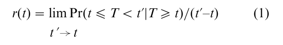
The transition rate provides a local, time-related description of how the process evolves over time. It can be interpreted as the propensity (or intensity) to change from an origin state to a destination state, at time t. But one should note that this propensity is defined in relation to a risk set (T≥t) at t, i.e., the set of units that still can experience the event because they have not yet had the event before t.

3.4 Statistical Models

The central idea in event history analysis is to make the transition rate, which describes a process evolving in time, dependent on time (t) and on a set of covariates, x:

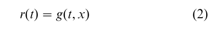
The causal interpretation of the transition rate requires that we take the temporal order in which the processes evolve very seriously. In other words, at any given point in time, t, the transition rate r(t) can be made dependent on conditions that happened to occur in the past (i.e., before t), but not on what is the case at t or in the future after t.

There are several possibilities to specify the functional relationship g (see Blossfeld and Rohwer 1995). For example, the exponential model, which normally serves as a baseline model, assumes that the transition rate can vary with different constellations of covariates x, but that the rates are time-constant. The piecewise constant exponential model allows the transition rate to vary across fixed time periods with period-specific effects of covariates. There are also different parametric models which are based on specific shapes of the time-dependence (e.g., the Gompertz-Makeham, Weibull, Sickle, Log-logistic, Log-normal, or Gamma model). If the time-shape of the base-line hazard rate is unspecified, and only possible effects of covariates x are estimated, the model is called a semi-parametric or partial likelihood model (Cox 1972). Finally, there are also models of unobserved heterogeneity in which the transition rate can be made dependent on the observed covariates x, the duration t, and a stochastic error term.

4. Parallel And Interdependent Processes

The most important scientific progress permitted by event history analysis is based on the opportunity to include explicitly measured time-varying covariates in transition rate models (see Blossfeld and Rohwer 1995). These covariates can change their values over process time in an analysis. Time-varying covariates can be qualitative or quantitative, and may stay constant for finite periods of time or change continuously. From a substantive point of view, time varying covariates can be conceptualized as observations of the sample path of parallel processes. These processes can operate at different levels. In sociology, for example, (a) there can be parallel processes at the level of the individual’s different domains of life (e.g., one may ask how upward and downward moves in an individual’s job career influence his her family trajectory); (b) there may be parallel processes at the level of some few individuals interacting with each other (e.g., one might study the effect of the career of the husband on his wife’s labor force participation); (c) there may be parallel processes at the intermediate level (e.g., one can analyze how organizational growth influences career advancement or changing household structure determines women’s labor force participation); (d) there may be parallel processes at the macro level (e.g., one may be interested in the effect of changes in the business cycle on family formation or career advancement); and (e) there may be any combination of such processes of type (a) to (d). For example, in the study of life-course, cohort and period effects, time-dependent covariates at different levels (see below) must be included simultaneously (multilevel analysis).

In dealing with such systems of parallel processes, the issue of reverse causation is often addressed in the methodological literature (see, e.g., Kalbfleisch and Prentice 1980, Tuma and Hannan 1984, Blossfeld et al. 1989, Yamaguchi 1991, Courgeau and Lelievre 1992). Reverse causation refers to the (direct or indirect) effect of the dependent process on the independent covariate process(es). Reverse causation is often seen as a problem because the effect of a time-dependent covariate on the transition rate is confounded with a feedback effect of the dependent process on the values of the time-dependent covariate. However, Blossfeld and Rohwer (1995) have developed a causal approach to the analysis of interdependent processes that also works in the case of interdependence, too. For example, if two interdependent processes, Y_t^A and Y_t^B, are given, a change in Y_t^A at any (specific) point in time t´ may be modeled as being depend on the history of both processes up to, but not including t´. Or stated in another way: what happens with Y_t^A at any point in time t is conditionally independent of what happens with Y_t^B at t´, conditional on the history of the joint process Y_t=(Y_t^A,Y_t^B) up to, but not including, t (‘principle of conditional independence’). Of course, the same reasoning can be applied if one focuses on Y_t^B instead of Y_t^A as the ‘dependent variable.’ Beginning with a transition rate model for the joint process, Y_t=(Y_t^A,Y^tB), and assuming the principle of conditional independence, the likelihood for this model can then be factorized into a product of the likelihoods for two separate models: a transition rate model for Y_t^A which is dependent on Y_t^B as a time-dependent covariate, and a transition rate model for Y_t^B, which is dependent on Y_t^A as a time-dependent covariate. From a technical point of view, there is therefore no need to distinguish between defined, ancillary, and internal covariates (see, e.g., Kalbfleisch and Prentice 1980) because all of these time-varying covariate types can be treated in the estimation procedure. Estimating the effects of time-varying processes on the transition rate can easily be achieved by applying the method of episode splitting (see Blossfeld and Rohwer 1995).

5. Unobserved Heterogeneity

Unfortunately, researchers are not always able to include all the important covariates into an event history analysis. These unobserved differences between subpopulations can lead to apparent time dependence at the population level and additional identification problems. There exists a fairly large literature on mis-specified models in general. In particular, there have been several proposals to deal with unobserved heterogeneity in transition rate models (so-called frailty models) (see, e.g., Blossfeld and Rohwer 1995).

6. Illustrative Applications

The following three applications illustrate the technical strength of event history models in different substantive contexts.

6.1 A Multi-Level Analysis Of Life-Course, Cohort, And Period Effects In Career Mobility

Any standard statistical analysis using age, year of birth (as a cohort measure), and chronological year of measurement (as a period measure) leads to an identification problem (age year of measurement– year of birth). The technical solution to that problem often is to assume that at least one of these measures is constant over time or to apply arbitrary statistical constraints. Blossfeld (1986) in an event history study of career mobility of German men approached this problem from a more substantive point of view. He suggested to rely more on explicit measures for the theoretically important macro effects of cohort and period and used 14 time series from official statistics indicating the long-term development of the labor market structure in Germany. Based on factor analysis, he first reduced the 14 highly correlated time series to two orthogonal macro factors which represented the ‘monotonic trend in the level of modernization’ and the ‘cyclic changes in labor market conditions’ and then matched these macro data to individual event career data to conduct a multi-level analysis. To represent the changing conditions under which cohorts enter the labor market, Blossfeld used the factor scores of these two factors at the year men entered the labor force. To introduce period as a time-dependent covariate, he used the method of episode splitting. In accordance with this method, the original job episodes were split into sub-episodes every year so that the factor scores of the two macro factors could be updated in each job episode for all employed men every year. Modeling cohort and period effects this way not only provides more direct and valid measures of the explanatory concepts, but also results in the disappearance of the problem of non-estimable parameters above. It was, therefore, not necessary to impose (in substantive terms normally unjustifiable) constraints on the parameters to identify life-course, cohort, and period effects.

6.2 Parallel Processes At The Le El Of The Individual: Women’s Rising Educational And Career Investments, And Changes In The Process Of Family Formation

Using event history models, Blossfeld and Huinink assessed the hypothesis of the ‘new home economics’ that women’s rising educational and career investments will lead to a decline in marriage and motherhood (see Blossfeld and Rohwer 1995, p. 143). Because the accumulation of educational and career resources is a lifetime process, they analyzed it as a dynamic process over the life course. To model the changes in the accumulation of qualifications over the life course, Blossfeld and Huinink updated a time-varying covariate ‘level of education’ at the age when a woman obtained a particular educational rank in the hierarchy. They also generated a time-dependent dummy variable indicating whether or not a woman is attending the educational system at a specific age. Finally, for the dynamic modeling of job-specific investments in human capital over the life course, Blossfeld and Huinink have developed a specific timedependent labor force experience measure, which they called ‘career resources.’ The time-dependent increments and final levels of this measure were designed to reflect the ‘quality of each job’ and the respective ‘employment durations.’ The time-dependent measure also took into account that career resources are declining when women interrupted their employment career. Blossfeld and Huinink applied the method of episode splitting to include these various time-dependent dimensions of education and career together with additional control variables in the rate equation. The results of their longitudinal analysis were surprising: contrary to the expectations of the economic approach to the family, women’s entry into marriage obviously was independent of women’s level of education and their career resources. Equally surprisingly, the effect of women’s level of education on the rate of their first birth was even positive. An explanation for the positive effect on the timing of first birth is easily demonstrated with an event history model: women who remain in school longer and attain high qualifications are first shifting their fertility decisions to higher ages, and then, they are subject to pressure not only from the potential increase in medical problems connected with having children late, but also from societal age norms. Thus the higher the educational attainment level the stronger the catching-up effect. This application demonstrates that the standard empirical support for the economic theory of the family claimed on the basis of cross-sectional data might be misleading. Cross-sectional data do not permit a differentiation between the time-dependent effect of accumulation of human capital over the life course and the time-dependent effect of participation in the educational system.

6.3 A Causal Approach To Interdependent Systems: The Effects Of Pregnancy On Entry Into Marriage For Couples Living In Consensual Unions

Finally, the application of a causal approach to interdependent systems is demonstrated by Blossfeld and Rohwer in an analysis of the effect of pregnancy on entry into marriage in Germany (see Blossfeld and Rohwer 1995, p. 157). This study shows that the effect of a fertility event on entry into marriage is highly time dependent: It starts to rise at some time shortly after conception (thus there is some time lag involved between cause and effect), increases during pregnancy to a maximum at around seven to eight months after conception, and then decreases again reaching a level even below the starting level at around six months after the birth of the child. Thus, the dynamic interdependence of fertility and nuptiality mainly occurs in a very specific phase of the life course and the unfolding effect of fertility on nuptiality is highly dynamic over time. Of course, standard statistical applications based on cross-sectional observation can be hardly used to analyse such situations in a meaningful way. However, in event history analysis, there is an easy way to approach that problem. One can use a series of time-dependent dummy variables each indicating a month since the occurrence of conception (the causal event). They show that the effects of the time-dependent dummy variable at first increase, reach a maximum, and then decrease again. Thus, starting with conception, there is an increasing normative pressure to avoid an illegitimate birth that increases the marriage rate, particularly for people who are already ‘ready for marriage.’ But with an increasing number of marriages, the composition of the group of still unmarried couples shifts towards couples being ‘less ready for marriage’ or being ‘not ready for marriage,’ which, of course, decreases the fertility effect again. This is an important result not only in substantive terms; the methodological lesson for event history analysis is also revealing. One should be very careful in modeling qualitative parallel processes with only one dummy variable (e.g., in the current application using only the time of conception, or the time of birth for the switch of the time-dependent covariate) because the effect itself might be highly time-dependent. For example, Blossfeld and Rohwer show that the fertility effect disappears completely, when the time-dependent covariate is switched at the time of birth because then a period with a low marriage rate up to the time of discovery of conception and a period with a high marriage rate during pregnancy is aggregated and compared with a period of low rate after the birth of the child.

Bibliography:

1. Andersen P K, Borgan Ø, Gill R D, Keiding N 1993 Statistical Models Based on Counting Processes. Springer-Verlag, New York
2. Blossfeld H-P 1986 Career opportunities in the Federal Republic of Germany: a dynamic approach to the study of life-course, cohort, and period eff European Sociological Review 2: 208–25
3. Blossfeld H-P, Hamerle A, Mayer K U 1989 Event History Analysis. Erlbaum, Hillsdale, NJ
4. Blossfeld H-P, Rohwer G 1995 Techniques of Event History Modeling. New Approaches to Causal Analysis. Erlbaum, Mahwah, NJ
5. Courgeau D, Lelievre E 1992 Event History Analysis in Demography. Clarendon, Oxford
6. Cox D R 1972 Regression models and life-tables. Journal of the Royal Statistics Society 34: 187–220
7. Kalbfleisch J D, Prentice R L 1980 The Statistical Analysis of Failure Time Data. Wiley, New York
8. Kaplan E L, Meier P 1958 Nonparametric estimation from incomplete observations. Journal of the American Statistical Association 53: 457–81
9. Lancaster T 1990 The Econometric Analysis of Transition Data. Cambridge University Press, Cambridge, UK
10. Tuma N B, Hannan M T 1984 Social Dynamics. Models and Methods. Academic Press, Orlando, FL
11. Vermunt J K 1997 Log-linear Models for Event Histories. Thousands Oakes, Newbury Park, CA
12. Yamaguchi K 1991 Event History Analysis. Sage, Newbury Park, CA